Unit 8: Working with heterogenous datasets and a view towards machine learning

1 Unit 8: Working with heterogenous datasets and a view towards machine learning

In this unit we learn how to deal with heterogenous datasets using data frames. We then explore basic concepts of machine learning. A deep dive into deep learning at UQ is in the STAT3007 course. Theory of machine learning (and statistical learning) is also studied in STAT3006. Other aspects of applied statistics and data analysis are studied in STAT3500. Our purpose with this unit is just to touch the tip of the iceberg on issues of data analysis and machine learning. The Julia language knowledge acquired in the previous units should help.

2 Databases

This course doesn’t touch databases, a rich topic of its own. (Do not confuse the term database with data structures or data frames). A database is a system that stores information in an organized and flexible manner. Many databases are relational databases and this means that they are comprised of multiple data tables that can be used together. The most common language for dealing with such databases is SQL. It is not a general programming language but rather a language for querying, modifying, and managing databases. At UQ you can study more about databases in the INFS2200 course as well as several other more advanced courses.

We now show you an example of database and a few things you may expect from SQL.

2.1 Relations

A “relation” is a mathematical term for a set over tuples (or named tuples), and is a generalization of a function.

For example, consider the function \(y = f(x)\). (The names here are \(x\) and \(y\)). An equivalent relation \(f\) can be constructed as a set of tuples of the form \((x, y)\). A particular tuple \((x, y)\) is in the relation \(f\) if and only if \(y = f(x)\).

Other things which are not strictly functions may be relations. For example, we can construct a relation of real numbers \((x, y)\) where \(x = y^2\). Or, equivalently, \(y = \pm\sqrt{x}\). Positive values of \(x\) correspond to two values of \(y\) (positive or negative square root). When \(x\) equals zero, there is only one solution for \(y\) (also zero). And for negative \(x\) there are no real \(y\) that satisfy the relation. Note that I say “relation” and not “function” here - functions are only a subset of relations.

Just like functions may have multiple inputs (\(x = f(a, b, c)\)), a relation may consist of tuples of any size (including zero!). And both functions and relations can exist over finite, discrete sets.

There are precisely two relations over tuples of size zero (i.e. \(()\)) - the empty relation, and the relation containing the empty tuple \(()\). You can use this fact to build up a kind of boolean logic in the language of relations, where the empty relation is false and the relation containing \(()\) is true.

Outside of mathematics, the kinds of relations normally modelled in databases are of the discrete, finite-sized variety. A relation over tuples \((a, b, c)\) is equivalent to table with three columns \(a\), \(b\) and \(c\). In a strictly relational databases, the ordering of the rows is irrelevant, and you cannot have two identical rows in the database (though in practice many databases in use may also deal with “bags” rather than “sets” of tuples, where rows can be repeated). The fields \(a\), \(b\) and \(c\) are drawn from their own set of possibilities, or datatype. For example, you might have (name, birthdate, is_adult) where name may be a string, birthdate may be a date, and is_adult may be a boolean.

name	birthdate	is_adult
"Alice"	2003-05-13	true
"Bob"	2005-12-10	false
"Charlie"	2004-09-21	true

Note that the latter two colums of this particular relation are a function if we assume is_adult is defined in terms of age (and thus in terms of birthdate).

In many relations, there are uniqueness constraints - for example the name might identify each row uniquely, or there may be a specific ID column to deal with different people sharing the same name. Such unique constraints are called “keys” and the primary identifier that you might use to fetch a particular row is called the “primary key”.

2.2 Relational schema

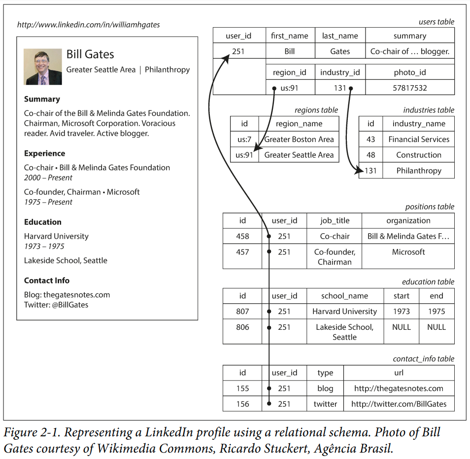
A single relation is a restrictive way to model your data. However, by allowing multiple relations, we can capture the various sets of data in the system, and piece them together by their relationships.

For example, each person in the table above might be related to other things. They might have jobs, bank accounts, etc. Within a single business a person might be a customer, a supplier and an employee, and for different purposes we might want data associated with that person (e.g. their birthdate might relate to advertizing promotions to customers, payrates for employees, etc).

Generally, to make keeping track of data easy, in a relational database you would store that person just once and create relationships between that person and other things. That way, if something changes about that person, it only needs to be updated in one place, and data remains consistent everywhere.

Here is an example of a more complex example - an imagining of how LinkedIn might store their data in a relational database (taken from “Designing Data-Intensive Applications” by Martin Kleppmann).

From Designing Data-Intensive Applications by Martin Kleppmann

2.3 SQL

The most popular way to interact with relational data is with via a language called SQL (originally “SEQUEL”, pronounced that way, backronymed to “structured query language”).

The language is from 1973 and doesn’t look like most other programming languages. With it, you declare a “query” and the database will find the best way to return the results. It is a form of declarative programming. Here is an example of getting some columns of data from the users table:

SELECT user_id, first_name, last_name
FROM users

You can filter the rows via a WHERE clause. Let’s say you knew the user_id for Bill Gates and you wanted just his data:

SELECT user_id, first_name, last_name
FROM users
WHERE user_id = 251

Data in different tables are related via the JOIN statement

SELECT users.user_id, first_name, last_name, organization
INNER JOIN positions ON positions.user_id = users.user_id
FROM users

Note we have to prefix the shared column names with the corresponding table (although in this case the difference is not particularly important, your query cannot be ambiguous).

But there is a problem here. This query would create a large amount of data, that the database would need to collect and send over the network to you. In the worst case, performing such a query could bring down a large system!

Generally, you have something more precise in mind. Like - which organizations has Bill Gates worked at?

SELECT users.user_id, first_name, last_name, organization
INNER JOIN positions ON positions.user_id = users.user_id
FROM users
WHERE users.user_id = 251

This will now return just two rows (for Microsoft, and the Bill & Melinda Gates Foundation), and is much less effort for the database, the network and the client. In real-world settings, complex joins could link data spanning dozens of tables.

There are several Julia libraries for interacting with SQL databases including the likes of LibPQ.jl allowing queries to be executed on a PostgreSQL database and the results returned as convenient Julia data structures. There’s even an SQL REPL in SQLRepl.jl if you want to execute SQL queries interactively and mix them with variables from your normal Julia session.

We won’t be writing SQL in this course but it is so pervasive in industry that is essential that you know that it exists and not to be afraid to use it! (It is a very useful and desirable skill!) All the relational data concepts expressed in SQL above also apply to in-memory data analysis using Julia and we show various examples of this next.

3 Dataframes

Working with tabular data is a central part of data analysis (think Excel). Data has rows (observations) and columns (variables/features). Typically a row would be for an individual, or item, or event. Typically a column would be for attributes of the individual, properties of the events, etc. Variables can be numerical, categorical, strings, or even more complex entities (e.g. images, arrays or dictionaries).

The datafile athlete_events.csv is a moderately sized dataset available from Kaggle covering all athletes that have participated the Summer or Winter Olympics between 1896 and 2016. The CSV file contains 40MB of data over 15 columns and more than 27,000 rows, which is “small data” for a modern computer (but would have been challenging in the 1980’s). In this context, “big data” is too large to be handled by a single machine, and we’ll discuss “big data” and “medium data” later.

You have already seen how to read and write from CSV files in Unit 3 where you also explored JSON files. You may recall using the DataFrames.jl package in that unit. We now take a deeper dive into the concept of dataframes.

We will use athlete_events.csv to show basic functionality of the DataFrames.jl and TypedTables.jl packages. In a sense these packages are alternatives. Seeing some functionality from each may be useful for gaining a general understanding of what to expect from such packages. If you work with Python, then using pandas is the common alternative. Similarly if you work with the R language then the built-in dataframes are common.

3.1 Basic data exploration

Whenever you receive a dataset, it takes some time to understand its contents. This process is generally known as “data exploration”. To do so, we generally load (a subset of) the data from disk and do some basic analysis in a Jupyter notebook or at the REPL.

We were introduced to CSV files earlier in the course. Here’s the first few lines of our file:

open("../data/athlete_events.csv") do io
   i = 0
   while i < 5
   println(readline(io))
   i += 1
   end
end

"ID","Name","Sex","Age","Height","Weight","Team","NOC","Games","Year","Season","City","Sport","Event","Medal"
"1","A Dijiang","M",24,180,80,"China","CHN","1992 Summer",1992,"Summer","Barcelona","Basketball","Basketball Men's Basketball",NA
"2","A Lamusi","M",23,170,60,"China","CHN","2012 Summer",2012,"Summer","London","Judo","Judo Men's Extra-Lightweight",NA
"3","Gunnar Nielsen Aaby","M",24,NA,NA,"Denmark","DEN","1920 Summer",1920,"Summer","Antwerpen","Football","Football Men's Football",NA
"4","Edgar Lindenau Aabye","M",34,NA,NA,"Denmark/Sweden","DEN","1900 Summer",1900,"Summer","Paris","Tug-Of-War","Tug-Of-War Men's Tug-Of-War","Gold"

The do syntax here injects a function which takes io::IO (an I/O stream for our file) into the first argument of the open function. It is syntax sugar. The open function is designed such that when the inner function returns or throws an error, open will automatically close the file to avoid resource leakage.

We can use the CSV.jl package to read the data and the DataFrames.jl package to hold the tabular data. We note in the above the appearance of "NA" for missing data, which we can use to help load the file.

using DataFrames, CSV
csv_file = CSV.File("../data/athlete_events.csv"; missingstring = "NA")
df = DataFrame(csv_file)
println("Data size: ", size(df))
println("Columns in the data: ", names(df))

Data size: (271116, 15)
Columns in the data: ["ID", "Name", "Sex", "Age", "Height", "Weight", "Team", "NOC", "Games", "Year", "Season", "City", "Sport", "Event", "Medal"]

Since the data is large, we don’t usually want to print it all. The first and last functions can be helpful:

first(df, 10)

10×15 DataFrame

Row	ID	Name	Sex	Age	Height	Weight	Team	NOC	Games	Year	Season	City	Sport	Event	Medal
	Int64	String	String1	Int64?	Int64?	Float64?	String	String3	String15	Int64	String7	String31	String31	String	String7?
1	1	A Dijiang	M	24	180	80.0	China	CHN	1992 Summer	1992	Summer	Barcelona	Basketball	Basketball Men's Basketball	missing
2	2	A Lamusi	M	23	170	60.0	China	CHN	2012 Summer	2012	Summer	London	Judo	Judo Men's Extra-Lightweight	missing
3	3	Gunnar Nielsen Aaby	M	24	missing	missing	Denmark	DEN	1920 Summer	1920	Summer	Antwerpen	Football	Football Men's Football	missing
4	4	Edgar Lindenau Aabye	M	34	missing	missing	Denmark/Sweden	DEN	1900 Summer	1900	Summer	Paris	Tug-Of-War	Tug-Of-War Men's Tug-Of-War	Gold
5	5	Christine Jacoba Aaftink	F	21	185	82.0	Netherlands	NED	1988 Winter	1988	Winter	Calgary	Speed Skating	Speed Skating Women's 500 metres	missing
6	5	Christine Jacoba Aaftink	F	21	185	82.0	Netherlands	NED	1988 Winter	1988	Winter	Calgary	Speed Skating	Speed Skating Women's 1,000 metres	missing
7	5	Christine Jacoba Aaftink	F	25	185	82.0	Netherlands	NED	1992 Winter	1992	Winter	Albertville	Speed Skating	Speed Skating Women's 500 metres	missing
8	5	Christine Jacoba Aaftink	F	25	185	82.0	Netherlands	NED	1992 Winter	1992	Winter	Albertville	Speed Skating	Speed Skating Women's 1,000 metres	missing
9	5	Christine Jacoba Aaftink	F	27	185	82.0	Netherlands	NED	1994 Winter	1994	Winter	Lillehammer	Speed Skating	Speed Skating Women's 500 metres	missing
10	5	Christine Jacoba Aaftink	F	27	185	82.0	Netherlands	NED	1994 Winter	1994	Winter	Lillehammer	Speed Skating	Speed Skating Women's 1,000 metres	missing

last(df, 10)

10×15 DataFrame

Row	ID	Name	Sex	Age	Height	Weight	Team	NOC	Games	Year	Season	City	Sport	Event	Medal
	Int64	String	String1	Int64?	Int64?	Float64?	String	String3	String15	Int64	String7	String31	String31	String	String7?
1	135565	Fernando scar Zylberberg	M	27	168	76.0	Argentina	ARG	2004 Summer	2004	Summer	Athina	Hockey	Hockey Men's Hockey	missing
2	135566	James Francis "Jim" Zylker	M	21	175	75.0	United States	USA	1972 Summer	1972	Summer	Munich	Football	Football Men's Football	missing
3	135567	Aleksandr Viktorovich Zyuzin	M	24	183	72.0	Russia	RUS	2000 Summer	2000	Summer	Sydney	Rowing	Rowing Men's Lightweight Coxless Fours	missing
4	135567	Aleksandr Viktorovich Zyuzin	M	28	183	72.0	Russia	RUS	2004 Summer	2004	Summer	Athina	Rowing	Rowing Men's Lightweight Coxless Fours	missing
5	135568	Olga Igorevna Zyuzkova	F	33	171	69.0	Belarus	BLR	2016 Summer	2016	Summer	Rio de Janeiro	Basketball	Basketball Women's Basketball	missing
6	135569	Andrzej ya	M	29	179	89.0	Poland-1	POL	1976 Winter	1976	Winter	Innsbruck	Luge	Luge Mixed (Men)'s Doubles	missing
7	135570	Piotr ya	M	27	176	59.0	Poland	POL	2014 Winter	2014	Winter	Sochi	Ski Jumping	Ski Jumping Men's Large Hill, Individual	missing
8	135570	Piotr ya	M	27	176	59.0	Poland	POL	2014 Winter	2014	Winter	Sochi	Ski Jumping	Ski Jumping Men's Large Hill, Team	missing
9	135571	Tomasz Ireneusz ya	M	30	185	96.0	Poland	POL	1998 Winter	1998	Winter	Nagano	Bobsleigh	Bobsleigh Men's Four	missing
10	135571	Tomasz Ireneusz ya	M	34	185	96.0	Poland	POL	2002 Winter	2002	Winter	Salt Lake City	Bobsleigh	Bobsleigh Men's Four	missing

This dataset appears to be sorted by last name. Each row corresponds to an entrant to an event. The ID column identifies each unique athlete.

A DataFrame is indexed like a 2D container of rows and columns. The : symbol means “all”.

df[1:10, :]

10×15 DataFrame

Row	ID	Name	Sex	Age	Height	Weight	Team	NOC	Games	Year	Season	City	Sport	Event	Medal
	Int64	String	String1	Int64?	Int64?	Float64?	String	String3	String15	Int64	String7	String31	String31	String	String7?
1	1	A Dijiang	M	24	180	80.0	China	CHN	1992 Summer	1992	Summer	Barcelona	Basketball	Basketball Men's Basketball	missing
2	2	A Lamusi	M	23	170	60.0	China	CHN	2012 Summer	2012	Summer	London	Judo	Judo Men's Extra-Lightweight	missing
3	3	Gunnar Nielsen Aaby	M	24	missing	missing	Denmark	DEN	1920 Summer	1920	Summer	Antwerpen	Football	Football Men's Football	missing
4	4	Edgar Lindenau Aabye	M	34	missing	missing	Denmark/Sweden	DEN	1900 Summer	1900	Summer	Paris	Tug-Of-War	Tug-Of-War Men's Tug-Of-War	Gold
5	5	Christine Jacoba Aaftink	F	21	185	82.0	Netherlands	NED	1988 Winter	1988	Winter	Calgary	Speed Skating	Speed Skating Women's 500 metres	missing
6	5	Christine Jacoba Aaftink	F	21	185	82.0	Netherlands	NED	1988 Winter	1988	Winter	Calgary	Speed Skating	Speed Skating Women's 1,000 metres	missing
7	5	Christine Jacoba Aaftink	F	25	185	82.0	Netherlands	NED	1992 Winter	1992	Winter	Albertville	Speed Skating	Speed Skating Women's 500 metres	missing
8	5	Christine Jacoba Aaftink	F	25	185	82.0	Netherlands	NED	1992 Winter	1992	Winter	Albertville	Speed Skating	Speed Skating Women's 1,000 metres	missing
9	5	Christine Jacoba Aaftink	F	27	185	82.0	Netherlands	NED	1994 Winter	1994	Winter	Lillehammer	Speed Skating	Speed Skating Women's 500 metres	missing
10	5	Christine Jacoba Aaftink	F	27	185	82.0	Netherlands	NED	1994 Winter	1994	Winter	Lillehammer	Speed Skating	Speed Skating Women's 1,000 metres	missing

Internally, a dataframe stores one vector of data per column. You can access any of them conveniently as “properties” with . syntax:

df.ID

271116-element Vector{Int64}:
      1
      2
      3
      4
      5
      5
      5
      5
      5
      5
      ⋮
 135566
 135567
 135567
 135568
 135569
 135570
 135570
 135571
 135571

df.Height

271116-element Vector{Union{Missing, Int64}}:
 180
 170
    missing
    missing
 185
 185
 185
 185
 185
 185
   ⋮
 175
 183
 183
 171
 179
 176
 176
 185
 185

As you can see from above, some data can be missing. How many heights are missing?

ismissing.(df.Height) |> count # Piping: `f(x) |> g` syntax means `g(f(x))`

60171

The count function counts the number of true values.

How many unique athletes are there?

unique(df.ID) |> length

135571

The unique operation has extra methods defined for DataFrames. We can get the athlete data like so:

athlete_df = unique(df, :ID)

135571×15 DataFrame

135546 rows omitted

Row	ID	Name	Sex	Age	Height	Weight	Team	NOC	Games	Year	Season	City	Sport	Event	Medal
	Int64	String	String1	Int64?	Int64?	Float64?	String	String3	String15	Int64	String7	String31	String31	String	String7?
1	1	A Dijiang	M	24	180	80.0	China	CHN	1992 Summer	1992	Summer	Barcelona	Basketball	Basketball Men's Basketball	missing
2	2	A Lamusi	M	23	170	60.0	China	CHN	2012 Summer	2012	Summer	London	Judo	Judo Men's Extra-Lightweight	missing
3	3	Gunnar Nielsen Aaby	M	24	missing	missing	Denmark	DEN	1920 Summer	1920	Summer	Antwerpen	Football	Football Men's Football	missing
4	4	Edgar Lindenau Aabye	M	34	missing	missing	Denmark/Sweden	DEN	1900 Summer	1900	Summer	Paris	Tug-Of-War	Tug-Of-War Men's Tug-Of-War	Gold
5	5	Christine Jacoba Aaftink	F	21	185	82.0	Netherlands	NED	1988 Winter	1988	Winter	Calgary	Speed Skating	Speed Skating Women's 500 metres	missing
6	6	Per Knut Aaland	M	31	188	75.0	United States	USA	1992 Winter	1992	Winter	Albertville	Cross Country Skiing	Cross Country Skiing Men's 10 kilometres	missing
7	7	John Aalberg	M	31	183	72.0	United States	USA	1992 Winter	1992	Winter	Albertville	Cross Country Skiing	Cross Country Skiing Men's 10 kilometres	missing
8	8	Cornelia "Cor" Aalten (-Strannood)	F	18	168	missing	Netherlands	NED	1932 Summer	1932	Summer	Los Angeles	Athletics	Athletics Women's 100 metres	missing
9	9	Antti Sami Aalto	M	26	186	96.0	Finland	FIN	2002 Winter	2002	Winter	Salt Lake City	Ice Hockey	Ice Hockey Men's Ice Hockey	missing
10	10	Einar Ferdinand "Einari" Aalto	M	26	missing	missing	Finland	FIN	1952 Summer	1952	Summer	Helsinki	Swimming	Swimming Men's 400 metres Freestyle	missing
11	11	Jorma Ilmari Aalto	M	22	182	76.5	Finland	FIN	1980 Winter	1980	Winter	Lake Placid	Cross Country Skiing	Cross Country Skiing Men's 30 kilometres	missing
12	12	Jyri Tapani Aalto	M	31	172	70.0	Finland	FIN	2000 Summer	2000	Summer	Sydney	Badminton	Badminton Men's Singles	missing
13	13	Minna Maarit Aalto	F	30	159	55.5	Finland	FIN	1996 Summer	1996	Summer	Atlanta	Sailing	Sailing Women's Windsurfer	missing
⋮	⋮	⋮	⋮	⋮	⋮	⋮	⋮	⋮	⋮	⋮	⋮	⋮	⋮	⋮	⋮
135560	135560	Stavroula Zygouri	F	36	171	63.0	Greece	GRE	2004 Summer	2004	Summer	Athina	Wrestling	Wrestling Women's Middleweight, Freestyle	missing
135561	135561	Frantiek Zyka	M	26	missing	missing	Czechoslovakia	TCH	1928 Summer	1928	Summer	Amsterdam	Athletics	Athletics Men's Marathon	missing
135562	135562	Milan Zyka	M	24	173	68.0	Czechoslovakia	TCH	1972 Summer	1972	Summer	Munich	Cycling	Cycling Men's Team Pursuit, 4,000 metres	missing
135563	135563	Olesya Nikolayevna Zykina	F	19	171	64.0	Russia	RUS	2000 Summer	2000	Summer	Sydney	Athletics	Athletics Women's 4 x 400 metres Relay	Bronze
135564	135564	Yevgeny Aleksandrovich Zykov	M	22	172	65.0	Russia-1	RUS	2002 Winter	2002	Winter	Salt Lake City	Luge	Luge Mixed (Men)'s Doubles	missing
135565	135565	Fernando scar Zylberberg	M	23	168	76.0	Argentina	ARG	2000 Summer	2000	Summer	Sydney	Hockey	Hockey Men's Hockey	missing
135566	135566	James Francis "Jim" Zylker	M	21	175	75.0	United States	USA	1972 Summer	1972	Summer	Munich	Football	Football Men's Football	missing
135567	135567	Aleksandr Viktorovich Zyuzin	M	24	183	72.0	Russia	RUS	2000 Summer	2000	Summer	Sydney	Rowing	Rowing Men's Lightweight Coxless Fours	missing
135568	135568	Olga Igorevna Zyuzkova	F	33	171	69.0	Belarus	BLR	2016 Summer	2016	Summer	Rio de Janeiro	Basketball	Basketball Women's Basketball	missing
135569	135569	Andrzej ya	M	29	179	89.0	Poland-1	POL	1976 Winter	1976	Winter	Innsbruck	Luge	Luge Mixed (Men)'s Doubles	missing
135570	135570	Piotr ya	M	27	176	59.0	Poland	POL	2014 Winter	2014	Winter	Sochi	Ski Jumping	Ski Jumping Men's Large Hill, Individual	missing
135571	135571	Tomasz Ireneusz ya	M	30	185	96.0	Poland	POL	1998 Winter	1998	Winter	Nagano	Bobsleigh	Bobsleigh Men's Four	missing

It keeps all columns of the first row containing each distinct ID, which will we take as representative (for their Sex, Height, Weight, etc).

3.2 Simple analysis

Now we are becoming familiar with the dataset, we might like to see what insights we can gain. For example, let’s see how many men and women have competed.

count(==("M"), athlete_df.Sex)  # `==(x)` creates a function `y -> y == x`

101590

count(==("F"), athlete_df.Sex)

33981

The count function is useful, but this gets tiresome for many “groups” of data. The SplitApplyCombine.jl package contains useful functions for grouping data.

using SplitApplyCombine

groupcount(athlete_df.Sex)

2-element Dictionaries.Dictionary{String1, Int64}:
 String1("M") │ 101590
 String1("F") │ 33981

Which allows us to explore larger sets of groupings:

# How many athletes by country
team_sizes = groupcount(athlete_df.Team)

1013-element Dictionaries.Dictionary{String, Int64}:
          "China" │ 2589
        "Denmark" │ 1840
 "Denmark/Sweden" │ 5
    "Netherlands" │ 2849
  "United States" │ 9051
        "Finland" │ 2271
         "Norway" │ 2029
        "Romania" │ 1735
        "Estonia" │ 336
         "France" │ 5717
                ⋮ │ ⋮
       "Sjovinge" │ 2
    "Brandenburg" │ 1
        "Struten" │ 1
       "Freia-19" │ 1
   "Luxembourg-1" │ 1
      "Sea Dog-2" │ 2
          "Mainz" │ 1
        "Druzhba" │ 1
        "China-3" │ 2

One of the most powerful tricks in data analysis is to sort your data.

sort(team_sizes)

1013-element Dictionaries.Dictionary{String, Int64}:
     "Nigeria-2" │ 1
 "Puerto Rico-2" │ 1
          "Lett" │ 1
       "Breslau" │ 1
  "Carabinier-5" │ 1
      "Evita VI" │ 1
      "Konstanz" │ 1
          "Nora" │ 1
          "Inca" │ 1
         "Snude" │ 1
               ⋮ │ ⋮
        "Sweden" │ 3598
     "Australia" │ 3731
         "Japan" │ 3990
       "Germany" │ 4318
        "Canada" │ 4504
         "Italy" │ 4650
 "Great Britain" │ 5706
        "France" │ 5717
 "United States" │ 9051

Note that groupcount is a specialization of the more flexible group(keys, values) function:

group(athlete_df.Team, athlete_df.Name)

1013-element Dictionaries.Dictionary{String, Vector{String}}:
          "China" │ ["A Dijiang", "A Lamusi", "Abudoureheman", "Ai Linuer", "Ai…
        "Denmark" │ ["Gunnar Nielsen Aaby", "Otto Mnsted Acthon", "Jesper Agerg…
 "Denmark/Sweden" │ ["Edgar Lindenau Aabye", "August Nilsson", "Gustaf Fredrik …
    "Netherlands" │ ["Christine Jacoba Aaftink", "Cornelia \"Cor\" Aalten (-Str…
  "United States" │ ["Per Knut Aaland", "John Aalberg", "Stephen Anthony Abas",…
        "Finland" │ ["Antti Sami Aalto", "Einar Ferdinand \"Einari\" Aalto", "J…
         "Norway" │ ["Kjetil Andr Aamodt", "Ragnhild Margrethe Aamodt", "Fritz …
        "Romania" │ ["Andreea Aanei", "Andrei Abraham", "Elisabeta Abrudeanu", …
        "Estonia" │ ["Evald rma (rman-)", "Meelis Aasme", "Moonika Aava", "Arvi…
         "France" │ ["Jamale (Djamel-) Aarrass (Ahrass-)", "Patrick Abada", "Re…
                ⋮ │ ⋮
       "Sjovinge" │ ["Christian Vinge", "Bengt Gran Waller"]
    "Brandenburg" │ ["Erik Johannes Peter Ernst von Holst"]
        "Struten" │ ["Knut Astrup Wang"]
       "Freia-19" │ ["Georges Camille Warenhorst"]
   "Luxembourg-1" │ ["Gza Wertheim"]
      "Sea Dog-2" │ ["Thomas Douglas Wynn Weston", "Joseph Warwick Wright"]
          "Mainz" │ ["Erich Wichmann-Harbeck"]
        "Druzhba" │ ["Valentin Alekseyevich Zamotaykin"]
        "China-3" │ ["Zhang Dan", "Zhang Hao"]

Rather than acting at the level of vectors, you can group an entire DataFrame into a GroupedDataFrame with the groupby function provided by DataFrames.jl:

gdf = groupby(athlete_df, :Team)

GroupedDataFrame with 1013 groups based on key: Team

First Group (2589 rows): Team = "China"

2564 rows omitted

Row	ID	Name	Sex	Age	Height	Weight	Team	NOC	Games	Year	Season	City	Sport	Event	Medal
	Int64	String	String1	Int64?	Int64?	Float64?	String	String3	String15	Int64	String7	String31	String31	String	String7?
1	1	A Dijiang	M	24	180	80.0	China	CHN	1992 Summer	1992	Summer	Barcelona	Basketball	Basketball Men's Basketball	missing
2	2	A Lamusi	M	23	170	60.0	China	CHN	2012 Summer	2012	Summer	London	Judo	Judo Men's Extra-Lightweight	missing
3	602	Abudoureheman	M	22	182	75.0	China	CHN	2000 Summer	2000	Summer	Sydney	Boxing	Boxing Men's Middleweight	missing
4	1463	Ai Linuer	M	25	160	62.0	China	CHN	2004 Summer	2004	Summer	Athina	Wrestling	Wrestling Men's Lightweight, Greco-Roman	missing
5	1464	Ai Yanhan	F	14	168	54.0	China	CHN	2016 Summer	2016	Summer	Rio de Janeiro	Swimming	Swimming Women's 200 metres Freestyle	missing
6	3605	An Weijiang	M	22	178	72.0	China	CHN	2006 Winter	2006	Winter	Torino	Speed Skating	Speed Skating Men's 500 metres	missing
7	3610	An Yulong	M	19	173	70.0	China	CHN	1998 Winter	1998	Winter	Nagano	Short Track Speed Skating	Short Track Speed Skating Men's 500 metres	Silver
8	3611	An Zhongxin	F	23	170	65.0	China	CHN	1996 Summer	1996	Summer	Atlanta	Softball	Softball Women's Softball	Silver
9	4639	Ao Changrong	M	25	173	71.0	China	CHN	2008 Summer	2008	Summer	Beijing	Hockey	Hockey Men's Hockey	missing
10	4641	Ao Tegen	M	21	181	90.0	China	CHN	1996 Summer	1996	Summer	Atlanta	Judo	Judo Men's Middleweight	missing
11	6376	Ba Dexin	M	23	185	80.0	China	CHN	2014 Winter	2014	Winter	Sochi	Curling	Curling Men's Curling	missing
12	6381	Ba Yan	F	21	183	78.0	China	CHN	1984 Summer	1984	Summer	Los Angeles	Basketball	Basketball Women's Basketball	Bronze
13	6382	Ba Yanchuan	M	24	187	100.0	China	CHN	1996 Summer	1996	Summer	Atlanta	Wrestling	Wrestling Men's Heavyweight, Greco-Roman	missing
⋮	⋮	⋮	⋮	⋮	⋮	⋮	⋮	⋮	⋮	⋮	⋮	⋮	⋮	⋮	⋮
2578	134870	Zhu Zhifu	M	25	179	72.0	China	CHN	2004 Summer	2004	Summer	Athina	Rowing	Rowing Men's Lightweight Double Sculls	missing
2579	134872	Zhuang Xiaoyan	F	23	173	98.0	China	CHN	1992 Summer	1992	Summer	Barcelona	Judo	Judo Women's Heavyweight	Gold
2580	134873	Zhuang Yong	F	16	172	68.0	China	CHN	1988 Summer	1988	Summer	Seoul	Swimming	Swimming Women's 100 metres Freestyle	Silver
2581	135230	Zong Xiangqing	M	24	193	72.0	China	CHN	1984 Summer	1984	Summer	Los Angeles	Fencing	Fencing Men's epee, Individual	missing
2582	135269	Zou Kai	M	20	158	55.0	China	CHN	2008 Summer	2008	Summer	Beijing	Gymnastics	Gymnastics Men's Individual All-Around	missing
2583	135270	Zou Shiming	M	23	165	49.0	China	CHN	2004 Summer	2004	Summer	Athina	Boxing	Boxing Men's Light-Flyweight	Bronze
2584	135271	Zou Sixin	M	25	178	76.0	China	CHN	1992 Summer	1992	Summer	Barcelona	Athletics	Athletics Men's Triple Jump	missing
2585	135272	Zou Wenzhi	M	missing	missing	missing	China	CHN	1948 Summer	1948	Summer	London	Football	Football Men's Football	missing
2586	135273	Zou Yuchen	M	20	203	107.0	China	CHN	2016 Summer	2016	Summer	Rio de Janeiro	Basketball	Basketball Men's Basketball	missing
2587	135274	Zou Zhenxian	M	28	184	72.0	China	CHN	1984 Summer	1984	Summer	Los Angeles	Athletics	Athletics Men's Triple Jump	missing
2588	135318	Zu Lijun	M	26	188	87.0	China	CHN	2016 Summer	2016	Summer	Rio de Janeiro	Swimming	Swimming Men's 10 kilometres Open Water	missing
2589	135445	Zuo Yue	M	21	192	88.0	China	CHN	1984 Summer	1984	Summer	Los Angeles	Volleyball	Volleyball Men's Volleyball	missing

⋮

Last Group (2 rows): Team = "China-3"

Row	ID	Name	Sex	Age	Height	Weight	Team	NOC	Games	Year	Season	City	Sport	Event	Medal
	Int64	String	String1	Int64?	Int64?	Float64?	String	String3	String15	Int64	String7	String31	String31	String	String7?
1	134439	Zhang Dan	F	16	167	48.0	China-3	CHN	2002 Winter	2002	Winter	Salt Lake City	Figure Skating	Figure Skating Mixed Pairs	missing
2	134461	Zhang Hao	M	17	181	72.0	China-3	CHN	2002 Winter	2002	Winter	Salt Lake City	Figure Skating	Figure Skating Mixed Pairs	missing

You can apply an operation to each group and bring the data together into a single DataFrame via the combine function.

combine(gdf, nrow => :Count)

1013×2 DataFrame

988 rows omitted

Row	Team	Count
	String	Int64
1	China	2589
2	Denmark	1840
3	Denmark/Sweden	5
4	Netherlands	2849
5	United States	9051
6	Finland	2271
7	Norway	2029
8	Romania	1735
9	Estonia	336
10	France	5717
11	Taifun	5
12	Morocco	459
13	Spain	2576
⋮	⋮	⋮
1002	Trintel II	1
1003	Springbok	1
1004	Monaco-1	1
1005	Sjovinge	2
1006	Brandenburg	1
1007	Struten	1
1008	Freia-19	1
1009	Luxembourg-1	1
1010	Sea Dog-2	2
1011	Mainz	1
1012	Druzhba	1
1013	China-3	2

The nrow => :Count syntax is a convenience provided by Dataframes.jl. We’ll explain how it works below.

3.3 Row- and column-based storage

What is a dataframe?

It is a data structure containing rows and columns. Internally it keeps each column of data as its own vector, which you can access as a property with .

athlete_df.Height

135571-element Vector{Union{Missing, Int64}}:
 180
 170
    missing
    missing
 185
 188
 183
 168
 186
    missing
   ⋮
 171
 172
 168
 175
 183
 171
 179
 176
 185

To construct a row, you need to grab the corresponding element from each vector.

first(eachrow(df))

DataFrameRow (15 columns)

Row	ID	Name	Sex	Age	Height	Weight	Team	NOC	Games	Year	Season	City	Sport	Event	Medal
	Int64	String	String1	Int64?	Int64?	Float64?	String	String3	String15	Int64	String7	String31	String31	String	String7?
1	1	A Dijiang	M	24	180	80.0	China	CHN	1992 Summer	1992	Summer	Barcelona	Basketball	Basketball Men's Basketball	missing

Or, you can use 2D indexing, as before

df[1, :]

DataFrameRow (15 columns)

Row	ID	Name	Sex	Age	Height	Weight	Team	NOC	Games	Year	Season	City	Sport	Event	Medal
	Int64	String	String1	Int64?	Int64?	Float64?	String	String3	String15	Int64	String7	String31	String31	String	String7?
1	1	A Dijiang	M	24	180	80.0	China	CHN	1992 Summer	1992	Summer	Barcelona	Basketball	Basketball Men's Basketball	missing

In this case there are 15 columns, so the computer must fetch data from 15 different places. This means that, for dataframes, operating with columns is faster than with rows. DataFrames are specialized for whole-of-table analytics, where each individual step in your analysis probably only involves a small number of columns.

There are other data structures you can use which store the data as rows. Most SQL databases will store their data like this. Traditional “transactional” databases are typically driven with reads and writes to one (or a few) rows at a time, and row-based storage is more efficient for such workloads. Some of the modern “analytics” databses will use column-based storage.

In Julia, perhaps the simplest such data structure is a Vector of NamedTuples. We can create one straightforwardly from a CSV.File:

NamedTuple.(csv_file)

271116-element Vector{NamedTuple{(:ID, :Name, :Sex, :Age, :Height, :Weight, :Team, :NOC, :Games, :Year, :Season, :City, :Sport, :Event, :Medal)}}:
 (ID = 1, Name = "A Dijiang", Sex = String1("M"), Age = 24, Height = 180, Weight = 80.0, Team = "China", NOC = String3("CHN"), Games = String15("1992 Summer"), Year = 1992, Season = String7("Summer"), City = String31("Barcelona"), Sport = String31("Basketball"), Event = "Basketball Men's Basketball", Medal = missing)
 (ID = 2, Name = "A Lamusi", Sex = String1("M"), Age = 23, Height = 170, Weight = 60.0, Team = "China", NOC = String3("CHN"), Games = String15("2012 Summer"), Year = 2012, Season = String7("Summer"), City = String31("London"), Sport = String31("Judo"), Event = "Judo Men's Extra-Lightweight", Medal = missing)
 (ID = 3, Name = "Gunnar Nielsen Aaby", Sex = String1("M"), Age = 24, Height = missing, Weight = missing, Team = "Denmark", NOC = String3("DEN"), Games = String15("1920 Summer"), Year = 1920, Season = String7("Summer"), City = String31("Antwerpen"), Sport = String31("Football"), Event = "Football Men's Football", Medal = missing)
 (ID = 4, Name = "Edgar Lindenau Aabye", Sex = String1("M"), Age = 34, Height = missing, Weight = missing, Team = "Denmark/Sweden", NOC = String3("DEN"), Games = String15("1900 Summer"), Year = 1900, Season = String7("Summer"), City = String31("Paris"), Sport = String31("Tug-Of-War"), Event = "Tug-Of-War Men's Tug-Of-War", Medal = String7("Gold"))
 (ID = 5, Name = "Christine Jacoba Aaftink", Sex = String1("F"), Age = 21, Height = 185, Weight = 82.0, Team = "Netherlands", NOC = String3("NED"), Games = String15("1988 Winter"), Year = 1988, Season = String7("Winter"), City = String31("Calgary"), Sport = String31("Speed Skating"), Event = "Speed Skating Women's 500 metres", Medal = missing)
 (ID = 5, Name = "Christine Jacoba Aaftink", Sex = String1("F"), Age = 21, Height = 185, Weight = 82.0, Team = "Netherlands", NOC = String3("NED"), Games = String15("1988 Winter"), Year = 1988, Season = String7("Winter"), City = String31("Calgary"), Sport = String31("Speed Skating"), Event = "Speed Skating Women's 1,000 metres", Medal = missing)
 (ID = 5, Name = "Christine Jacoba Aaftink", Sex = String1("F"), Age = 25, Height = 185, Weight = 82.0, Team = "Netherlands", NOC = String3("NED"), Games = String15("1992 Winter"), Year = 1992, Season = String7("Winter"), City = String31("Albertville"), Sport = String31("Speed Skating"), Event = "Speed Skating Women's 500 metres", Medal = missing)
 (ID = 5, Name = "Christine Jacoba Aaftink", Sex = String1("F"), Age = 25, Height = 185, Weight = 82.0, Team = "Netherlands", NOC = String3("NED"), Games = String15("1992 Winter"), Year = 1992, Season = String7("Winter"), City = String31("Albertville"), Sport = String31("Speed Skating"), Event = "Speed Skating Women's 1,000 metres", Medal = missing)
 (ID = 5, Name = "Christine Jacoba Aaftink", Sex = String1("F"), Age = 27, Height = 185, Weight = 82.0, Team = "Netherlands", NOC = String3("NED"), Games = String15("1994 Winter"), Year = 1994, Season = String7("Winter"), City = String31("Lillehammer"), Sport = String31("Speed Skating"), Event = "Speed Skating Women's 500 metres", Medal = missing)
 (ID = 5, Name = "Christine Jacoba Aaftink", Sex = String1("F"), Age = 27, Height = 185, Weight = 82.0, Team = "Netherlands", NOC = String3("NED"), Games = String15("1994 Winter"), Year = 1994, Season = String7("Winter"), City = String31("Lillehammer"), Sport = String31("Speed Skating"), Event = "Speed Skating Women's 1,000 metres", Medal = missing)
 ⋮
 (ID = 135566, Name = "James Francis \"Jim\" Zylker", Sex = String1("M"), Age = 21, Height = 175, Weight = 75.0, Team = "United States", NOC = String3("USA"), Games = String15("1972 Summer"), Year = 1972, Season = String7("Summer"), City = String31("Munich"), Sport = String31("Football"), Event = "Football Men's Football", Medal = missing)
 (ID = 135567, Name = "Aleksandr Viktorovich Zyuzin", Sex = String1("M"), Age = 24, Height = 183, Weight = 72.0, Team = "Russia", NOC = String3("RUS"), Games = String15("2000 Summer"), Year = 2000, Season = String7("Summer"), City = String31("Sydney"), Sport = String31("Rowing"), Event = "Rowing Men's Lightweight Coxless Fours", Medal = missing)
 (ID = 135567, Name = "Aleksandr Viktorovich Zyuzin", Sex = String1("M"), Age = 28, Height = 183, Weight = 72.0, Team = "Russia", NOC = String3("RUS"), Games = String15("2004 Summer"), Year = 2004, Season = String7("Summer"), City = String31("Athina"), Sport = String31("Rowing"), Event = "Rowing Men's Lightweight Coxless Fours", Medal = missing)
 (ID = 135568, Name = "Olga Igorevna Zyuzkova", Sex = String1("F"), Age = 33, Height = 171, Weight = 69.0, Team = "Belarus", NOC = String3("BLR"), Games = String15("2016 Summer"), Year = 2016, Season = String7("Summer"), City = String31("Rio de Janeiro"), Sport = String31("Basketball"), Event = "Basketball Women's Basketball", Medal = missing)
 (ID = 135569, Name = "Andrzej ya", Sex = String1("M"), Age = 29, Height = 179, Weight = 89.0, Team = "Poland-1", NOC = String3("POL"), Games = String15("1976 Winter"), Year = 1976, Season = String7("Winter"), City = String31("Innsbruck"), Sport = String31("Luge"), Event = "Luge Mixed (Men)'s Doubles", Medal = missing)
 (ID = 135570, Name = "Piotr ya", Sex = String1("M"), Age = 27, Height = 176, Weight = 59.0, Team = "Poland", NOC = String3("POL"), Games = String15("2014 Winter"), Year = 2014, Season = String7("Winter"), City = String31("Sochi"), Sport = String31("Ski Jumping"), Event = "Ski Jumping Men's Large Hill, Individual", Medal = missing)
 (ID = 135570, Name = "Piotr ya", Sex = String1("M"), Age = 27, Height = 176, Weight = 59.0, Team = "Poland", NOC = String3("POL"), Games = String15("2014 Winter"), Year = 2014, Season = String7("Winter"), City = String31("Sochi"), Sport = String31("Ski Jumping"), Event = "Ski Jumping Men's Large Hill, Team", Medal = missing)
 (ID = 135571, Name = "Tomasz Ireneusz ya", Sex = String1("M"), Age = 30, Height = 185, Weight = 96.0, Team = "Poland", NOC = String3("POL"), Games = String15("1998 Winter"), Year = 1998, Season = String7("Winter"), City = String31("Nagano"), Sport = String31("Bobsleigh"), Event = "Bobsleigh Men's Four", Medal = missing)
 (ID = 135571, Name = "Tomasz Ireneusz ya", Sex = String1("M"), Age = 34, Height = 185, Weight = 96.0, Team = "Poland", NOC = String3("POL"), Games = String15("2002 Winter"), Year = 2002, Season = String7("Winter"), City = String31("Salt Lake City"), Sport = String31("Bobsleigh"), Event = "Bobsleigh Men's Four", Medal = missing)

The above constructs a NamedTuple for each row of the CSV file and and returns it as a Vector.

This is a great data structure that you can use “out of the box” with no packages, and your “everyday” analysis work will usually be fast so long as you do not have many, many columns.

If you want to use an identical interface with row-based storage, there is the TypedTables package. In this package, a Table is an AbstractArray{<:NamedTuple}, each column is stored as its own vector, and when you index the table table[i] it assembles the row as a NamedTuple for you.

using TypedTables
Table(csv_file)

Table with 15 columns and 271116 rows:
      ID  Name                  Sex  Age  Height   Weight   Team            ⋯
    ┌────────────────────────────────────────────────────────────────────────
 1  │ 1   A Dijiang             M    24   180      80.0     China           ⋯
 2  │ 2   A Lamusi              M    23   170      60.0     China           ⋯
 3  │ 3   Gunnar Nielsen Aaby   M    24   missing  missing  Denmark         ⋯
 4  │ 4   Edgar Lindenau Aabye  M    34   missing  missing  Denmark/Sweden  ⋯
 5  │ 5   Christine Jacoba Aa…  F    21   185      82.0     Netherlands     ⋯
 6  │ 5   Christine Jacoba Aa…  F    21   185      82.0     Netherlands     ⋯
 7  │ 5   Christine Jacoba Aa…  F    25   185      82.0     Netherlands     ⋯
 8  │ 5   Christine Jacoba Aa…  F    25   185      82.0     Netherlands     ⋯
 9  │ 5   Christine Jacoba Aa…  F    27   185      82.0     Netherlands     ⋯
 10 │ 5   Christine Jacoba Aa…  F    27   185      82.0     Netherlands     ⋯
 11 │ 6   Per Knut Aaland       M    31   188      75.0     United States   ⋯
 12 │ 6   Per Knut Aaland       M    31   188      75.0     United States   ⋯
 13 │ 6   Per Knut Aaland       M    31   188      75.0     United States   ⋯
 14 │ 6   Per Knut Aaland       M    31   188      75.0     United States   ⋯
 15 │ 6   Per Knut Aaland       M    33   188      75.0     United States   ⋯
 16 │ 6   Per Knut Aaland       M    33   188      75.0     United States   ⋯
 17 │ 6   Per Knut Aaland       M    33   188      75.0     United States   ⋯
 ⋮  │ ⋮            ⋮             ⋮    ⋮      ⋮        ⋮           ⋮         ⋱

Sometimes plain vectors or (typed) tables may be more convenient or faster than dataframes, and sometimes dataframes will be more convenient and faster than plain vectors or typed tables. Another popular approach is to use Query.jl. For your assessment you may use whichever approach you like best.

3.4 DataFrames

For now we will double-down on DataFrames.jl.

Here is a nice cheatsheet for the syntax of DataFrames, and I recommend downloading and possibly even printing it out for your convenience.

3.4.1 Constructing dataframes

A DataFrame can be constructed directly from data columns.

df = DataFrame(a = [1, 2, 3], b = [2.0, 4.0, 6.0])

3×2 DataFrame

Row	a	b
	Int64	Float64
1	1	2.0
2	2	4.0
3	3	6.0

You can get or set columns to the dataframe with . property syntax.

df.a

3-element Vector{Int64}:
 1
 2
 3

df.c = ["A", "B", "C"]
df

3×3 DataFrame

Row	a	b	c
	Int64	Float64	String
1	1	2.0	A
2	2	4.0	B
3	3	6.0	C

3.4.2 Indexing dataframes

A dataframe is indexed a bit like a 2D matrix - the first index is the row and the second is the column.

df[1, :c]

"A"

The :c here is a Symbol, which is a kind of “compiler string”. The compiler stores the names of your types, fields, variables, modules and functions as Symbol. In fact, the syntax df.c is just sugar for getproperty(df, :c). You can get multiple rows and/or columns.

df[1, :]

DataFrameRow (3 columns)

Row	a	b	c
	Int64	Float64	String
1	1	2.0	A

df[:, :c]

3-element Vector{String}:
 "A"
 "B"
 "C"

df[1:2, [:a, :c]]

2×2 DataFrame

Row	a	c
	Int64	String
1	1	A
2	2	B

3.4.3 Filtering dataframes

The filter function returns a collection where the elements satisfy some predicate function (i.e. a function that returns a Bool). We can grab just the odd-numbered rows from df by running filter over each row.

filter(row -> isodd(row.a), df)

2×3 DataFrame

Row	a	b	c
	Int64	Float64	String
1	1	2.0	A
2	3	6.0	C

Unfortunately, in this case this is quite inefficient. For each row the program must

1. construct a DataFrameRow
2. access the a field dynamically
3. compute isodd

This is slower than we’d like because the compiler doesn’t really know what columns are in a DataFrame (or a DataFrameRow) and what type they may be. Every time we do step 2 there is a lot of overhead.

To fix this problem DataFrames.jl introduced special syntax of the form:

filter(:a => isodd, df)

2×3 DataFrame

Row	a	b	c
	Int64	Float64	String
1	1	2.0	A
2	3	6.0	C

This will automatically extract the :a column just once and use it to construct a fast & fully compiled predicate function. Another way to think about how this works is via indexing:

df[isodd.(df.a), :]

2×3 DataFrame

Row	a	b	c
	Int64	Float64	String
1	1	2.0	A
2	3	6.0	C

So first we find:

isodd.(df.a)

3-element BitVector:
 1
 0
 1

And afterwards we take a subset of the rows.

df[[1,3], :]

2×3 DataFrame

Row	a	b	c
	Int64	Float64	String
1	1	2.0	A
2	3	6.0	C

3.4.4 select and transform

You can grab one-or-more columns via select:

select(df, [:a, :c])

3×2 DataFrame

Row	a	c
	Int64	String
1	1	A
2	2	B
3	3	C

The columns can be modified or even renamed as a part of this process. This is more useful with transform, which keeps the existing columns and lets you add new ones:

using Statistics
transform(df, :b => mean => :mean_b)

3×4 DataFrame

Row	a	b	c	mean_b
	Int64	Float64	String	Float64
1	1	2.0	A	4.0
2	2	4.0	B	4.0
3	3	6.0	C	4.0

You can read this as “take column b, do mean on it, and put the result in column mean_b”. A new dataframe is constructed, and df is unmodified.

Note that the transformation applies to whole columns. If you want to transform just a single row at a time, wrap the function in a ByRow.

transform!(df, :a => ByRow(isodd) => :a_isodd, :c => ByRow(lowercase) => :c_lowercase)

3×5 DataFrame

Row	a	b	c	a_isodd	c_lowercase
	Int64	Float64	String	Bool	String
1	1	2.0	A	true	a
2	2	4.0	B	false	b
3	3	6.0	C	true	c

Here we used transform! (note the !) which mutates df.

3.4.5 groupby and combine

The groupby function will group a DataFrame into a collection of SubDataFrames:

gdf = groupby(df, :a_isodd)

GroupedDataFrame with 2 groups based on key: a_isodd

First Group (1 row): a_isodd = false

Row	a	b	c	a_isodd	c_lowercase
	Int64	Float64	String	Bool	String
1	2	4.0	B	false	b

⋮

Last Group (2 rows): a_isodd = true

Row	a	b	c	a_isodd	c_lowercase
	Int64	Float64	String	Bool	String
1	1	2.0	A	true	a
2	3	6.0	C	true	c

You can combine these together by applying a bulk transformation to each group

combine(gdf, :b => sum, :c => join)

2×3 DataFrame

Row	a_isodd	b_sum	c_join
	Bool	Float64	String
1	false	4.0	B
2	true	8.0	AC

This is known as the split-apply-combine strategy, and the pattern comes up frequently.

3.4.6 innerjoin

We won’t use this a lot in this course, but you can perform a relational join between dataframes with the innerjoin function. (Note that the join function is for joining strings together into longer strings)

names_df = DataFrame(ID = [1, 2, 3], Name = ["John Doe", "Jane Doe", "Joe Blogs"])

3×2 DataFrame

Row	ID	Name
	Int64	String
1	1	John Doe
2	2	Jane Doe
3	3	Joe Blogs

jobs = DataFrame(ID = [1, 2, 4], Job = ["Lawyer", "Doctor", "Farmer"])

3×2 DataFrame

Row	ID	Job
	Int64	String
1	1	Lawyer
2	2	Doctor
3	4	Farmer

DataFrames.innerjoin(names_df, jobs; on = :ID)

2×3 DataFrame

Row	ID	Name	Job
	Int64	String	String
1	1	John Doe	Lawyer
2	2	Jane Doe	Doctor

Only rows with matching :IDs are kept.

3.5 More analysis

Now that we know a little bit more about the tools, let’s use them to see what insights we can glean from our Olympic athlete data.

3.5.1 Athlete height

We can see that, on average, male competitors are taller than female competitors.

mean(athlete_df.Height[athlete_df.Sex .== "M"])

missing

Oops. Not all athletes have a Height attribute.

mean(skipmissing(athlete_df.Height[athlete_df.Sex .== "M"]))

179.43963320733585

mean(skipmissing(athlete_df.Height[athlete_df.Sex .== "F"]))

168.9320099255583

The males are a bit more than 10cm taller, on average.

OK, now let’s perform a slightly more complex analysis. We will answer the question - has athlete height has changed over time? What do you think?

We can plot the average height as a function of Year. To see how to do that, first we’ll repeat the above using the tools of DataFrames.jl:

athlete_by_gender = groupby(athlete_df, :Sex)
combine(athlete_by_gender, :Height => mean ∘ skipmissing => :Height)

2×2 DataFrame

Row	Sex	Height
	String1	Float64
1	M	179.44
2	F	168.932

Given that, it’s pretty straightforward to do this as a function of year.

using Plots
athlete_by_year = groupby(athlete_df, :Year)
height_by_year = combine(athlete_by_year, :Height => mean ∘ skipmissing => :Height)
plot(height_by_year.Year, height_by_year.Height, ylim = [155, 182]; ylabel = "Height (cm)", xlabel = "Year", legend = false)

This doesn’t show anything interesting. Yet. There are a few confounding factors to eliminate first.

First, there is something going on strange with the years, which started at 4-year increments and changed to 2-year increments. This is due to Winter Olympics moving to a different year to the Summer Olympics in 1994.

athlete_by_games = groupby(athlete_df, [:Year, :Season])
height_by_games = combine(athlete_by_games, :Height => mean ∘ skipmissing => :Height)
plot(height_by_games.Year, height_by_games.Height, ylim = [155, 182]; ylabel = "Height (cm)", xlabel = "Year", group = height_by_games.Season, legend = :bottomright)

The type of sport might affect the height of the competitors (think basketball players vs jockeys) so it’s good to split these groups. Here it seems that winter competitors are slightly shorter than summer competitors.

The second confounding factor is that women have increasingly became a larger fraction of the competitors at the Olympics, so we will split also by gender.

athlete_by_cohort = groupby(athlete_df, [:Year, :Season, :Sex])
height_by_cohort = combine(athlete_by_cohort, :Height => mean ∘ skipmissing => :Height)
plot(height_by_cohort.Year, height_by_cohort.Height, ylim = [155, 182]; ylabel = "Height (cm)", xlabel = "Year", group = tuple.(height_by_cohort.Season, height_by_cohort.Sex), legend = :bottomright)

Whoa! Now we clearly see that heights have trended up at least 5cm since 1900!

What’s going on here? I suspect it is a combination of several facts:

1. On average, people born before the end of World War 2 were shorter, due to nutritional changes.
2. Sport has become more elite and competitive over the years, and height may correlate with success in many Olympic sports.
3. Women competitors have become more prevalent over time, reducing the average height of all competitors.
4. Similarly, winter competitors may have become more prevalent over time, who appear to be shorter than the summer cohorts.

We can easily verify #3 above.

gender_by_games = combine(athlete_by_games, :Sex => (s -> count(==("F"), s) / length(s)) => :Fraction_Female)
plot(gender_by_games.Year, gender_by_games.Fraction_Female, ylim = [0, 1]; ylabel = "Fraction female", xlabel = "Year", group = gender_by_games.Season, legend = :topright)

Note that we could have given up our analysis with the first plot, above, and arrived at completely the wrong conclusion!

Having these tools under your belt is a very useful skill. It is quite common that you need to have the skills to dig under the surface to get a correct understanding of data. It is just as useful to debunk a myth or assumption as it is to find a hitherto unknown correlation.

3.5.2 Histograms

These are just the means, we can also compare the statistic distribution (for the 2016 games, say):

histogram(collect(skipmissing(athlete_by_cohort[(2016, "Summer", "M")].Height)), xlabel = "Height (cm)", opacity = 0.5, label = "Male")
histogram!(collect(skipmissing(athlete_by_cohort[(2016, "Summer", "F")].Height)), opacity = 0.5, label = "Female")

The histogram function is useful for identifying features of distributions (e.g. if it is bimodal).

3.5.3 Further questions

We could analyse this data another hundred ways. Some questions that come to mind are:

• How does team success relate to socioeconomic indicators of their home country, such as GDP per capita? Do richer countries do comparatively better than poorer countries? To do this, we would need to join the data with country data.
• Does team success depend on the distance between the host of the Olympics and the home nation? For example, Australia received a lot of medals during the Sydney 2000 Olympics.
• Can we predict how well a team will do at a given Olympics, based on data like above? This is heading in the direction of machine learning.

3.6 Fitting linear models

Here we’ll briefly show how to fit linear models to your data using the package GLM.jl. A one dimensional linear model may be written

\[ Y = \beta_0 + \beta_1 X + \epsilon \]

where \(Y\) is some dependent variable to be predicted, \(X\) is the independent variable and \(\epsilon\) is some random noise. The task of fitting is to estimate the model parameters \(\beta_0\) and \(\beta_1\); one may also want to estimate the variance of the noise \(\epsilon\). Simple linear models like this (and the multidimensional generalization) can be fit with least squares to give the maximum liklihood estimate of the parameters \(\beta\).

Let’s look at a simple example from the athletes data

using GLM, Underscores

df = DataFrame(CSV.File("../data/athlete_events.csv"; missingstring = "NA"))

rowing_by_year = @_ df |> 
   groupby(__, [:Year, :Sport]) |>
   combine(__, nrow => :Count) |>
   sort(__, :Year) |>
   filter(:Sport => ==("Rowing"), __)

model = lm(@formula(Count ~ Year), rowing_by_year)

scatter(rowing_by_year.Year, rowing_by_year.Count, label="Data")
plot!(rowing_by_year.Year, predict(model, rowing_by_year), label="Prediction")

Q: Is this linear fit a reasonable thing to do? (What’s going on after 2000?)

Let’s now look at how to fit a multidimensional model using GLM.jl. In the multidimensional case we have several independent variables \(X_1, \dots, X_p\) and several dependent variables \(Y_1, \dots, Y_n\):

\[ Y_i = \beta_0 + \beta_1 X_{i1} + \beta_2 X_{i2} + \dots \beta_p X_{ip} + \epsilon_i \]

Here’s an example of fitting CPU performance for some historical CPUs, taken from the book “Statistics with Julia”:

using RDatasets, Statistics

df = dataset("MASS", "cpus")
df.Freq = map( x->10^9/x , df.CycT)

model = lm(@formula(Perf ~ MMax + Cach + ChMax + Freq), df)
println("n = ", size(df)[1])
println("(Avg,Std) of observed performance: ", (mean(df.Perf),std(df.Perf)))
model

n = 209
(Avg,Std) of observed performance: (105.61722488038278, 160.83058719907774)

StatsModels.TableRegressionModel{LinearModel{GLM.LmResp{Vector{Float64}}, GLM.DensePredChol{Float64, LinearAlgebra.CholeskyPivoted{Float64, Matrix{Float64}, Vector{Int64}}}}, Matrix{Float64}}

Perf ~ 1 + MMax + Cach + ChMax + Freq

Coefficients:
───────────────────────────────────────────────────────────────────────────────────
                    Coef.   Std. Error      t  Pr(>|t|)     Lower 95%     Upper 95%
───────────────────────────────────────────────────────────────────────────────────
(Intercept)  -46.5763      7.62382      -6.11    <1e-08  -61.6078      -31.5447
MMax           0.00841457  0.000639214  13.16    <1e-28    0.00715426    0.00967489
Cach           0.872508    0.152825      5.71    <1e-07    0.571189      1.17383
ChMax          0.96736     0.234847      4.12    <1e-04    0.504321      1.4304
Freq           9.74951e-7  5.5502e-7     1.76    0.0805   -1.1936e-7     2.06926e-6
───────────────────────────────────────────────────────────────────────────────────

Using the model to predict:

pred(x) = round(coef(model)'*vcat(1,x), digits = 3)
println("Estimated performance test computers: for computer A: ", pred([32000, 32, 32, 4*10^7]))

# Using the data and the `predict()` function
test_data = DataFrame(
   name  = ["Computer A", "Computer B"],
   MMax  = [32000,        32000],
   Cach  = [32,           16],
   ChMax = [32,           32],
   Freq  = [4*10^7,       6*10^7],
)

println("Estimated performance test computers:")
println(predict(model, test_data))

Estimated performance test computers: for computer A: 320.564
Estimated performance test computers:
Union{Missing, Float64}[320.56388734263373, 326.1027664254048]

Note that GLM stands for “generalized linear model” and the GLM.jl package can fit more general models - specifically those where the left and right hand sides are related by a nonlinear “link function”, and where the random noise is not normally distributed.

4 Memory management in data workflows

Generally in data heavy workflows we have three rough “sizes” to worry about.

1. Small data: data fits in RAM. Just load it up and process it all at once. We are doing this in this course.
2. Medium data: data is too big for RAM, but it fits on disk. Incrementally load “chunks” from disk, save the results, and load the next chunk, etc - known as “out-of-core” processing. Multiple such steps might be required in a “pipeline”. Reading and writing to disk is slower than RAM, and processing might take so long that restarting from scratch (after a fault or power blackout, for example) is not realistic, so you generally need to be able to save and restore your intermediate state, or update your data incrementally. A typical SQL database is in this category, handling the persistence, fault-tolerance and pipelining for you automatically.
3. Big data: data is too big to fit on the hard drive of a single computer. Generally requires a distributed solution for both storage and processing. At this scale, it is “business as usual” for computers to die and hard drives or RAM to corrupt, and you can’t have your multi-million-dollar operation brought down by a single rogue bitflip. These days it is common and convenient to use cloud services for these situations - like those provided by Amazon (AWS), Microsoft (Azure) or Google (GCP).

The boundaries between these regimes depends on your computer hardware. As you get step up, the complexity increases rapidly, especially with respect to fault tolerance.

At my previous job with Fugro we processed petabytes of LiDAR, imagery and positioning data to create a 3D model of the world. We used AWS to store and index the data, as well as process it. The effort in “data engineering” was as much as was required in the “data science”. Generally, it pays to have your data sorted out before attempting any higher-order analytics at scale (such as machine learning, below).