To introduce things say you have an array of values and want to find the maximal value. How would you do it? Here is some Julia code:
usingRandom# Make the program generate the same data every time it runsRandom.seed!(42)functionfind_max(data) max_value =-Inffor x in dataif x > max_value max_value = xendendreturn max_valueendRandom.seed!(0)data =rand(100)max_value =find_max(data)println("Found maximal value: $(max_value)")
Found maximal value: 0.9972781130627076
Here is a question: How many times was a new maximum found?
Let’s count.
usingRandomfunctionfind_max(data) max_value =-Inf n =0for x in dataif x > max_value n = n+1 max_value = xendendreturn (max_value, n)endRandom.seed!(0)data =rand(100)(max_value, n) =find_max(data)println("Found maximal value: $(max_value)")println("There were $n records along the way.")
Found maximal value: 0.9972781130627076
There were 7 records along the way.
But for different data (different seed) obviously there are a different number of possible records…
Random.seed!(1)data =rand(100)max_value, n =find_max(data)println("Found maximal value: $(max_value)")println("There were $n records along the way.")
Found maximal value: 0.9894764460236303
There were 10 records along the way.
How many on average? Denote the number of records for \(n\) data points by \(X_n\) then, \[
X_n = I_1 + I_2 + \ldots + I_n,
\] where, \[
I_i =
\begin{cases}
1 & \text{if}~i~\text{'th data point is a record}, \\
0 & \text{otherwise}.
\end{cases}
\] Now, \[
{\mathbb E}[X_n] = {\mathbb E}[I_1] + {\mathbb E}[I_2] + \ldots + {\mathbb E}[I_n].
\] Observe that \({\mathbb E}[I_i] = {\mathbb P}(I_i = 1)\) and for statistically independent and identically distributed data points we have, \[
{\mathbb P}(I_i = 1) = \frac{1}{i},
\] why?
Hence, \[
{\mathbb E}[X_n] = h_n = \sum_{i=1}^n \frac{1}{i},
\] the harmonic sum. It is known that \[
h_n = \log(n) + \gamma + o(1),
\] where \(\gamma\) is the Euler–Mascheroni constant and \(o(1)\) is a term that vanishes as \(n \to \infty\). That is \[
h_n \approx \log(n) + \gamma.
\] Let’s see it…
usingPlotsprintln("γ = $(Float64(MathConstants.γ))") #\gamma + [TAB]h(n) =sum(1/i for i in1:n)approx_h(n) =log(n) +MathConstants.γfor n in1:10println("$(n)\t$(h(n))\t$(approx_h(n))")enderr = [h(n) -approx_h(n) for n in1:20]scatter(1:20, err, xticks=1:20, xlabel="n", ylabel ="Error", ylim = (0, 0.5), legend=false)
Here is a Monte Carlo estimate and a histogram of the distribution:
usingStatisticsrecords = []for s in1:10^5Random.seed!(s) data =rand(100) (_, n) =find_max(data)push!(records, n)endprintln("log(100) + γ = $(approx_h(100)), Monte Carlo Estimate: $(mean(records))")histogram(records, ticks =1:maximum(records), normed=true, xlabel="n", ylabel="probability", legend=false)
log(100) + γ = 5.182385850889625, Monte Carlo Estimate: 5.19232
2 Preamble (before really getting into code)
Here is some general information to discuss before getting to the nitty gritty.
2.1 What we assume you “already know”
You are coming to this course after doing several mathematics and statistics courses. Hence we assume you have already done some coding or scripting of sorts. For example you might have done a bit of Python, some MATLAB scripting, used some code in R, or similar. In all these cases, we assume that you’ve already experienced a bit of the following:
You have written some commands/code that are later interpreted by the computer to execute actions.
You are aware that in a computer program you typically define variables; often giving them meaningful names.
You know that you can make computers do the same action again and again, by wrapping code in loops, often using conditional statements (if) to decide how the program should continue.
You have even used and/or written a few functions (or routines) where you specify how some action should be done and describe that action in a function.
You certainly know how to use files, directories, and the internet.
Finally, you are also somewhat of a mathematician. You have done courses such as STAT1301 (first year stats), MATH1071 (Analysis + Linear Algebra) + MATH1072 (Mutivariable Calculus + some modelling) + several more math electives.
Wikipedia says this about a computer: > A computer is a machine that can be programmed to carry out sequences of arithmetic or logical operations automatically.
Ada
We can live with this definition. Here are some notes and bits.
Most computers today implement some form of the von Neumann architecture. It means there are processing units (CPUs), memory, external (slower) storage, and multiple input out mechanisms. There are multiple forms to this but in most cases the following components exist:
A set of instructions is executed via hardware. The instructions are sometimes themselves encoded in hardware, but are often written in software and can be changed.
There is memory, and often multiple forms of memory. Fast memory near the CPU (cache), RAM (Random Access Memory) allowing the CPU to compute, disk memory, and even more memory (almost infinite) on the internet.
There are often higher order abstractions that organize the way instructions are executed by the CPU(s). This is typically an operating system (Linux, Mac OS, Windows, iOS, Android, etc…).
You should also know of the conceptual mathematical model of a computer which is typically the Turing machine. The nice thing about such an abstraction is that it often helps understand what and how certain algorithms operate, as well as their limitations. There are also related computer theoretic notions such as Finite Automata. We don’t get too much into such computer science/discrete math notions in the course. However, it is very interesting stuff, that lies at the centre of mathematics and computer science.
Alan Turing
2.4 The culture of software development and Who is a programmer?
Two software aphorisms to consider as you progress:
“code is read much more often than it is written”
“There are only two hard things in Computer Science: cache invalidation and naming things”
Some general observations of the teething difficulties of working in software as a mathematician:
Big complaint of software engineers interacting with mathematicians is “black box of code that isn’t easy to follow”.
In academia, code is an artifact of doing research work. Outside academia code is the output.
If code was treated like writing a paper (or was a research output valued by itself), this transition would be smoother.
Mathematicians can bring value at many levels of an organisation, as you will be interacting with a diverse set of people. Communication skills are important, so treat code as one way of communicating.
2.5 Historical Ladder of delegation in programming (a Faustian bargain)
Rung
You gain
You give up
Machine code
Full control over the machine
Impossible to write anything of real complexity
Assembly
Human-readable mnemonics, more expressive
Still brutal to write anything complex, tied to one machine
Floating point†
Tractable arithmetic on real numbers
Exactness - rounding error, (a+b)+c ≠ a+(b+c)
Compiled
Source portable, even more expressive
Still low-level - you manage memory yourself
Dynamic / interpreted
Machine fully abstracted away, very expressive
Speed
JIT
Expressive and fast
Predictability† - performance depends on runtime behaviour in ways that are hard to reason about
Parallel / concurrent
Scale beyond one core
Deterministic execution order† - race conditions, results that depend on scheduling
Libraries
Enormous leverage, don’t reinvent the wheel
Must fit its opinions, lose visibility into what’s actually happening
Classical ML
Solves problems too complex to hand-specify
Exact specification† - “correct” becomes statistical, not provable
LLMs
Extraordinary generality, near-natural-language interface to computation
Specification and implementation control, determinism† - no contract like a compiler gives you, output is plausible, not guaranteed
† same flavour of bargain each time, trading a guarantee (exact bits, order, correctness) for capability. Floating point started this thread decades before anyone was worried about AI.
2.6 Bits, bytes, hex, binary, and the works…
A bit is either \(0\) or \(1\). A byte is a sequence of \(8\) bits. Hence there are \(2^8 = 256\) options.
If you use a byte to encode an integer, then one option is the range \(0,1,2,\ldots,255\). This is called an unsigned integer, or UInt8 in Julia.
Another option is the range \(-127,\ldots,128\) (still \(256\) possibilities) and this is called an Int8.
println("Unsigned 8 bit integers\n")println("Number \tBinary \tHexadecimal\tJulia representation")for n in0:255if n ≤18|| n ≥250#\le + [TAB], \ge + [TAB]println("$(lpad(string(n), 3)):\t$(bitstring(UInt8(n)))\t$(lpad(string(n, base =16), 2))\t\t$(repr(UInt8(n)))")elseif n ∈19:21#in(n,19:21) \in + [TAB]println("\t ⋮")endend
Unsigned 8 bit integers

Number  Binary      Hexadecimal Julia representation
  0:    00000000     0      0x00
  1:    00000001     1      0x01
  2:    00000010     2      0x02
  3:    00000011     3      0x03
  4:    00000100     4      0x04
  5:    00000101     5      0x05
  6:    00000110     6      0x06
  7:    00000111     7      0x07
  8:    00001000     8      0x08
  9:    00001001     9      0x09
 10:    00001010     a      0x0a
 11:    00001011     b      0x0b
 12:    00001100     c      0x0c
 13:    00001101     d      0x0d
 14:    00001110     e      0x0e
 15:    00001111     f      0x0f
 16:    00010000    10      0x10
 17:    00010001    11      0x11
 18:    00010010    12      0x12
       ⋮
       ⋮
       ⋮
250:    11111010    fa      0xfa
251:    11111011    fb      0xfb
252:    11111100    fc      0xfc
253:    11111101    fd      0xfd
254:    11111110    fe      0xfe
255:    11111111    ff      0xff
println("Signed 8 bit integers (observe the sign bit)\n")println("Number \tBinary")for n in-128:127if n ∈-128:-120|| n ∈-5:5|| n ∈125:127println("$(lpad(n, 4)):\t$(bitstring(Int8(n)))")elseif n ∈-119:-117|| n ∈6:8println("\t ⋮")endend
Base \(16\), called hexadecimal is very common. One hexadecimal character uses four bits. The prefix notation 0x prior to the digits often indicates a number is represented as hexadecimal. The digit symbols
usingLaTeXStrings, Randomprintln("The digits:")print("Hex:\t")[print(string(n, base =16), n<10 ? " ":" ") for n in0:15];println()print("Decimal:")data = [0x0, 0x1, 0x2, 0x3, 0x4, 0x5, 0x6, 0x7, 0x8, 0x9, 0xa, 0xb, 0xc, 0xd, 0xe, 0xf][print(n, " ") for n in data];println("\n\nSome random values:")Random.seed!(1)for _ in1:5 x =rand(UInt8)println("In decimal (base 10): $x,\t In hex (base 16): $(string(x,base=16))")end
The digits:
Hex:    0 1 2 3 4 5 6 7 8 9 a  b  c  d  e  f
Decimal:0 1 2 3 4 5 6 7 8 9 10 11 12 13 14 15

Some random values:
In decimal (base 10): 18,    In hex (base 16): 12
In decimal (base 10): 89,    In hex (base 16): 59
In decimal (base 10): 178,   In hex (base 16): b2
In decimal (base 10): 160,   In hex (base 16): a0
In decimal (base 10): 234,   In hex (base 16): ea
You can also use the prefix notation 0b to denote binary
x =11@show (x ==0b1011) @show (x ==0xb);
x == 0x0b = true
x == 0x0b = true
You can do arithmetic on any base. Specifically for hex and binary.
Sometimes you need to keep in mind that types have a finite range and arithmetic will wrap around.
println("Wrap-around of unsigned integers")x =UInt8(255)@show xprintln("Adding 1: ", x +UInt8(1), "\n")println("Wrap-around of signed integers")x =Int8(127)@show xprintln("Adding 1: ", x +Int8(1), "\n" )println("A \"Normal\" integer") x =UInt(0xffffffffffffffff) #Note that UInt = UInt64 on 64 bit computers @show xprintln("Adding 1: ", x +1, "\n")
Wrap-around of unsigned integers
x = 0xff
Adding 1: 0

Wrap-around of signed integers
x = 127
Adding 1: -128

A "Normal" integer
x = 0xffffffffffffffff
Adding 1: 0
Why does this occur? A useful exercise is to examine how addition can be implemented purely using logical operations (as occurs in hardware). Consider the following code
half_adder(a::Bool, b::Bool) = (xor(a,b), a & b)functionfull_adder(a::Bool, b::Bool, carry::Bool) (s1, carry_a) =half_adder(a, b) (s2, carry_b) =half_adder(s1, carry)return (s2, carry_a | carry_b)endfunctionadd_n_digits(a::Int, b::Int, n)#calculate y = a + b using array indexing and logic operations#convert to a vector of booleans a_bool =digits(Bool, a, base =2, pad = n) b_bool =digits(Bool, b, base =2, pad = n) y_bool =fill(Bool(0), n) carry =falsefor i =1: n (y_bool[i], carry) =full_adder(a_bool[i], b_bool[i], carry)endreturn y_bool, a_bool, b_boolend#turn boolean array back into a stringdisplay_bool_array(y) =join(reverse(Int.(y)), "")a =1b =1y_bool, a_bool, b_bool =add_n_digits(a, b, 16)println("adding $a + $b")println("a = $(display_bool_array(a_bool))")println("b = $(display_bool_array(b_bool))")println("y = $(display_bool_array(y_bool))", "\n")a =1b =2^16-1#biggest 16 bit UInty_bool, a_bool, b_bool =add_n_digits(a, b, 16)println("adding $a + $b")println("a = $(display_bool_array(a_bool))")println("b = $(display_bool_array(b_bool))")println("y = $(display_bool_array(y_bool))", "\n")
adding 1 + 1
a = 0000000000000001
b = 0000000000000001
y = 0000000000000010

adding 1 + 65535
a = 0000000000000001
b = 1111111111111111
y = 0000000000000000
It is a useful exercise to consider how an equivalent logic based approach might work for other seemingly simple operations such as multiplication. Also, consider how many discrete operations are required, as the size of the binary representation increases.
Binary data considered as a string can often appear as hex.
# Hello World!println("There is more than one way to say hello:")# This is an array consisting of three stringshelloArray = ["Hello","G'day","Shalom"]for i in1:3println("\t", helloArray[i], " World!")endprintln("\nThese squares are just perfect:")# This construct is called a 'comprehension' (or 'list comprehension')squares = [i^2 for i in0:10]# You can loop on elements of arrays without having to use indexingfor s in squaresprint(" ",s)endprintln()# The last line of every code snippet is also evaluated as output (in addition to# any figures and printing output generated previously).sqrt.(squares)
There is more than one way to say hello:
    Hello World!
    G'day World!
    Shalom World!

These squares are just perfect:
  0  1  4  9  16  25  36  49  64  81  100
The “quakeIII” algorithm for the reciprocal of square root Float32
sqrt(25)
5.0
x =sqrt(2)@show x, x^2x =sqrt(2f0) #32 bit float (Float32)@show x, x^2
(x, x ^ 2) = (1.4142135623730951, 2.0000000000000004)
(x, x ^ 2) = (1.4142135f0, 1.9999999f0)
(1.4142135f0, 1.9999999f0)
sqrt(-1)
DomainError with -1.0:
sqrt was called with a negative real argument but will only return a complex result if called with a complex argument. Try sqrt(Complex(x)).
Stacktrace:
[1] throw_complex_domainerror(f::Symbol, x::Float64) @Base.Math./math.jl:33
[2] sqrt @./math.jl:627 [inlined]
[3] sqrt(x::Int64) @Base.Math./math.jl:1546
[4] top-level scope
@~/github/ProgrammingCourse-with-Julia-SimulationAnalysisAndLearningSystems/quarto/lecture-unit-2.qmd:493
sqrt(Complex(-1))
0.0 + 1.0im
√2#\sqrt + [TAB]
1.4142135623730951
In Julia a function (such as sqrt or its alias √) can have many methods:
How can we compute the square root if we didn’t have the sqrt() function? Of course one answer is to use another in-built alternative:
x =36@show x^0.5
x ^ 0.5 = 6.0
6.0
But how is such an algorithm implemented? In Julia’s source code, in math.jl you’ll find the following in lines 647-650:
@inline function sqrt(x::Union{Float32,Float64})
    x < zero(x) && throw_complex_domainerror(:sqrt, x)
    sqrt_llvm(x)
end
Here sqrt_llvm() compiles to Low Level Virtual Machine(LLVM), so while many functions in Julia are actually implemented in Julia, with square roots it is better to let the underlying low level (LLVM) code handle square roots because it is later changed to assembly code; which is very fast. You can inspect this via the macros @code_llvm and @code_native.
This will generally look the same on different computer types (LLVM is hardware agnostic):
@code_llvmsqrt(2.5)
; Function Signature: sqrt(Float64); @ math.jl:626 within `sqrt`definedouble@julia_sqrt_20323(double %"x::Float64") #0 {top:; @ math.jl:627 within `sqrt`; ┌ @ float.jl:623 within `<`
%0 = fcmpugedouble %"x::Float64", 0.000000e+00; └bri1 %0, label%L5, label%L3L3:; preds = %topcallvoid@j_throw_complex_domainerror_20326(ptrnonnull@"jl_sym#sqrt#20327.jit", double %"x::Float64") #11
unreachableL5:; preds = %top; @ math.jl:628 within `sqrt`
%1 = calldouble@llvm.sqrt.f64(double %"x::Float64")retdouble %1
}
This will look different for different computer types (cpus):
One method is the Babylonian algorithm: Say we are given a positive real number \(z\) and want its square root. We start with an initial guess \(x_0\). We then apply the recursive step,
\[
x_{k+1} = \frac{1}{2}\Big(x_k+\frac{z}{x_k}\Big).
\] That is, at each step the next iterate is the arithmetic mean of the previous iterate, \(x_k\), and \(z/x_k\). The Babylonian algorithm runs this iteration until convergence (note the default initial guess in this implementation is \(z/2\)):
functionbab_sqrt(z ; init_x = z/2, verbose =false, tol =1e-10) x = init_xwhiletrue verbose &&println("Babylonian iterate: $x") next_x =0.5*(x + z / x)abs(next_x - x) < tol &&break x = next_xend xendbs, s =bab_sqrt(5000;verbose =true), sqrt(5000)println("Babylonian:\t$bs\nSystem:\t\t$s")
We can view the ancient Babylonian method as an application of the more general Newton’s method for solving equations. Our goal is to solve \(x^2 = z\) where \(z\) is given and \(x\) is desired. That is define \(f(x) = x^2 - z\) and we wish to find the solution of \(f(x) = 0\). Newton’s method iterates,
\[
x_{k+1} = x_k - \frac{f(x_k)}{f'(x_k)},
\]
based on an affine (linear) approximation of \(f(\cdot)\) at the point \(x_k\). Here \(f'(\cdot)\) is the derivative, which in our case is \(f'(x) = 2x\). So Newton’s iterates for finding the square root are,
Sometimes we are not just interested in computing the \(\sqrt{z}\), but rather,
\[
\frac{1}{\sqrt{z}}.
\]
A common case for that is when we have a vector, say \(u = [u_1, u_2]\) and we wish to create the normalized (unit \(L_2\) norm) vector,
\[
\overline{u} = \frac{1}{\|u\|} u = \frac{1}{\sqrt{u_1^2 + u_2^2}} u.
\]
We could obviously just compute the reciprocal \(1/\sqrt{z}\) by dividing by \(1\), for example in the case of the vector normalization we can do this in Julia in multiple ways:
usingLinearAlgebrau = [1,1] #A vector pointing in a 45 degree angle up.uN1 =normalize(u) #Julia has a function for this in linear algebra.@show uN1uN2 = u/norm(u) #Here we do it via the norm() function@show uN2uN3 = u/sqrt(u'u) # Note that u'u = u_1^2 + u_2^2 (the inner product)@show uN3uN4 = u/sqrt(u[1]^2+ u[2]^2)@show uN4uN5 = u/sqrt(dot(u,u))@show uN5;
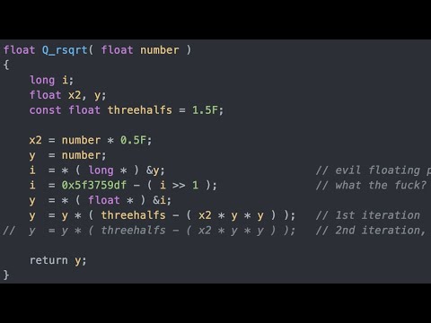
However for the interest of it, lets consider another way to do it which is specific for 32bit floating point numbers: The Fast Inverse Square Root Algorithm. This is how the original code appeared in the C Language.
float Q_rsqrt( float number )
{
    long i;
    float x2, y;
    const float threehalfs = 1.5F;

    x2 = number * 0.5F;
    y  = number;
    i  = * ( long * ) &y;                       // evil floating point bit level hacking
    i  = 0x5f3759df - ( i >> 1 );               // what the f___?
    y  = * ( float * ) &i;
    y  = y * ( threehalfs - ( x2 * y * y ) );   // 1st iteration
//  y  = y * ( threehalfs - ( x2 * y * y ) );   // 2nd iteration, this can be removed

    return y;
}
Here is the equivalent code in Julia.
functionfast_inv_sqrt(number::Float32) x2 =number*Float32(0.5)#reinterpret the float32 number to a 32 bit unsigned integer i =reinterpret(UInt32, number)#do WTF magic i =0x5f3759df- (i >>1)#reinterpet back into a float32 y =reinterpret(Float32, i)#do an iteration of newtons method from a good first guess y = y * (Float32(1.5) - (x2 * y^2))return yendx =Float32(4.0)y =fast_inv_sqrt(x)print("1/√(4) ≈ $(y)")
1/√(4) ≈ 0.49915358
Click the image below to watch a video with a detailed explanation of the algorithm:
Fast Inverse Square Root
3.4 Factorial (the 2’nd story)
Basics
Recursion
BigInts
The Gamma function
Accuracy of the Stirling approximation (will use arrays also for plotting)
A few basic ways to compute \(10! = 1\cdot 2 \cdot \ldots \cdot 10\):
\[
n! =
\begin{cases}
n \cdot (n-1)! & n = 1,2,\ldots\\
1 & n = 0.
\end{cases}
\]
This is a recursive definition. Let’s implement it:
functionmy_factorial(n)if n ==0return1elsereturn n *my_factorial(n -1)endendmy_factorial(10)
3628800
Let’s see what happens with this recursion:
functionmy_factorial(n)println("Calling my_factorial($n)")if n ==0 ret_val =1else ret_val = n *my_factorial(n -1)endprintln("Returning from the call of my_factorial($n)") ret_valendmy_factorial(10)
Calling my_factorial(10)
Calling my_factorial(9)
Calling my_factorial(8)
Calling my_factorial(7)
Calling my_factorial(6)
Calling my_factorial(5)
Calling my_factorial(4)
Calling my_factorial(3)
Calling my_factorial(2)
Calling my_factorial(1)
Calling my_factorial(0)
Returning from the call of my_factorial(0)
Returning from the call of my_factorial(1)
Returning from the call of my_factorial(2)
Returning from the call of my_factorial(3)
Returning from the call of my_factorial(4)
Returning from the call of my_factorial(5)
Returning from the call of my_factorial(6)
Returning from the call of my_factorial(7)
Returning from the call of my_factorial(8)
Returning from the call of my_factorial(9)
Returning from the call of my_factorial(10)
Here is the my_factorial() function (written compactly).
my_factorial(n) = n ==0 ? 1: n *my_factorial(n-1)my_factorial(10)
3628800
Such compact writing does not change what actually happens under the hood. To see this consider both forms:
my_factorial1(n) = n ==0 ? 1: n *my_factorial1(n -1)functionmy_factorial2(n)if n ==0return1elsereturn n *my_factorial2(n -1)endend
my_factorial2 (generic function with 1 method)
And use Julia’s @code_lowered macro to see how Julia parses the code into an intermediate representation (before being further compiled to LLVM). In both forms we get the exact same intermediate form.
How large can factorials we compute be? With BigInt, created via big(), there is sometimes no limit, but if we wanted to stay within the machine word size, we stay with Int64 (with Julia Int is either Int32 on “32 bit machines” or Int64 on “64 bit machines). But even 32 bit machines support 64 bit integers (by doubling words).
Lets first use Stirling’s approximation to get an estimate of the largest factorial we can compute with UInt64.
To see the approximation isn’t unreasonable, observe that \(n! \le n^n\) (why?) but isn’t so far either.
#An array of named tuples (note that "n!" is just a name)[(n_fact =factorial(n), n_pow_n = n^n, ratio =factorial(n) / (n^n)) for n in1:10]
10-element Vector{@NamedTuple{n_fact::Int64, n_pow_n::Int64, ratio::Float64}}:
 (n_fact = 1, n_pow_n = 1, ratio = 1.0)
 (n_fact = 2, n_pow_n = 4, ratio = 0.5)
 (n_fact = 6, n_pow_n = 27, ratio = 0.2222222222222222)
 (n_fact = 24, n_pow_n = 256, ratio = 0.09375)
 (n_fact = 120, n_pow_n = 3125, ratio = 0.0384)
 (n_fact = 720, n_pow_n = 46656, ratio = 0.015432098765432098)
 (n_fact = 5040, n_pow_n = 823543, ratio = 0.006119899021666143)
 (n_fact = 40320, n_pow_n = 16777216, ratio = 0.00240325927734375)
 (n_fact = 362880, n_pow_n = 387420489, ratio = 0.000936656708416885)
 (n_fact = 3628800, n_pow_n = 10000000000, ratio = 0.00036288)
The other \(\sqrt{n} e^{-n}\) factor of \(n\) in Stirling, corrects for this and \(\sqrt{2 \pi}\) is a constant.
stirling(n) = (√(2π*n))*(n/MathConstants.e)^n [ ( n! =factorial(n), stirling =stirling(n), ratio =round(factorial(n) /stirling(n), digits =5), ) for n in1:10]
10-element Vector{@NamedTuple{n!::Int64, stirling::Float64, ratio::Float64}}:
 (n! = 1, stirling = 0.9221370088957891, ratio = 1.08444)
 (n! = 2, stirling = 1.9190043514889832, ratio = 1.04221)
 (n! = 6, stirling = 5.836209591345864, ratio = 1.02806)
 (n! = 24, stirling = 23.506175132893294, ratio = 1.02101)
 (n! = 120, stirling = 118.0191679575901, ratio = 1.01678)
 (n! = 720, stirling = 710.078184642185, ratio = 1.01397)
 (n! = 5040, stirling = 4980.395831612462, ratio = 1.01197)
 (n! = 40320, stirling = 39902.39545265671, ratio = 1.01047)
 (n! = 362880, stirling = 359536.87284194835, ratio = 1.0093)
 (n! = 3628800, stirling = 3.5986956187410373e6, ratio = 1.00837)
So let’s use Stirling to see how big \(n\) can be to fit in UInt64. That is solve \[
\sqrt{2 \pi} \, n^{n+\frac{1}{2}} e^{-n} = 2^{64}-1.
\] There are multiple ways to try to do this. We’ll use floating point numbers and just search. Observe this:
2^64-1, typeof(2^64-1) #This is a signed integer by default
Here is the search (to simplify let’s focus on signed integers):
limit =typemax(Int64)n =1whilestirling(n) <= limitglobal n +=1endn -=1#why is this here? What can be done instead?println("Found maximal n for n! with 64 bits to be $n.")
Found maximal n for n! with 64 bits to be 20.
Let’s try it:
factorial(20)
2432902008176640000
What about \(n=21\)?
factorial(21)
OverflowError: 21 is too large to look up in the table; consider using `factorial(big(21))` instead
Stacktrace:
[1] factorial_lookup @./combinatorics.jl:26 [inlined]
[2] factorial(n::Int64) @Base./combinatorics.jl:34
[3] top-level scope
@~/github/ProgrammingCourse-with-Julia-SimulationAnalysisAndLearningSystems/quarto/lecture-unit-2.qmd:861
Indeed \(n=21\) doesn’t fit within the 64 bit limit. However as suggested by the error message, using big() can help:
typeof(big(21))
BigInt
factorial(big(21))
51090942171709440000
With (software) big integers everything goes:
n =10^3big_stuff =factorial(big(n));num_digits =Int(ceil(log10(big_stuff))) println("The facotrial of $n has $num_digits decimal digits.")
The facotrial of 1000 has 2568 decimal digits.
What about factorials of numbers that aren’t positive integers?
factorial(6.5)
MethodError: no method matching factorial(::Float64)
The function `factorial` exists, but no method is defined for this combination of argument types.
Closest candidates are:
factorial(::UInt128)
@Basecombinatorics.jl:33
factorial(::Int128)
@Basecombinatorics.jl:32
factorial(::BigFloat)
@Basempfr.jl:855
...
Stacktrace:
[1] top-level scope
@~/github/ProgrammingCourse-with-Julia-SimulationAnalysisAndLearningSystems/quarto/lecture-unit-2.qmd:886
No, that isn’t defined. But you may be looking for the gamma special function:
\[
\Gamma(z)=\int_{0}^{\infty} x^{z-1} e^{-x} d x.
\]
usingSpecialFunctions#You'll need to add (install) SpecialFunctionsgamma(6.5)
287.88527781504433
To feel more confident this value agrees with the integral definition of \(\Gamma(\cdot)\); let’s compute the integral in a very crude manner (Riemann_sum):
functionmy_crude_gamma(z; delta=0.01, M =50)integrand(x) = x^(z-1)*exp(-x) x_grid =0:delta:Msum(delta*integrand(x) for x in x_grid)endmy_crude_gamma(6.5)
287.88527781504325
Now note that the gamma function is sometimes considered as the continuous version of the factorial because, \[
\begin{aligned}
\Gamma(z+1) &=\int_{0}^{\infty} x^{z} e^{-x} d x \\
&=\left[-x^{z} e^{-x}\right]_{0}^{\infty}+\int_{0}^{\infty} z x^{z-1} e^{-x} d x \\
&=\lim _{x \rightarrow \infty}\left(-x^{z} e^{-x}\right)-\left(-0^{z} e^{-0}\right)+z \int_{0}^{\infty} x^{z-1} e^{-x} d x \\
&=z \, \Gamma(z).
\end{aligned}
\]
That is, the recursive relationship \(\Gamma(z+1) = z\Gamma(z)\) holds similarly to \(n! = n \cdot (n-1)!\). Further \[
\Gamma(1) = \int_0^\infty e^{-x} \, dx = 1.
\] Hence we see that for integer \(z\), \(\Gamma(z) = (z-1)!\) or \(n! = \Gamma(n+1)\). Let’s try this.
usingSpecialFunctions[(n = n, n! =factorial(n), Γ =gamma(n+1)) for n in0:10]
The gamma function can also be extended outside of the positive reals. At some points it isn’t defined though.
@showgamma(-1.1) #here defined.gamma(-1) #here not defined
gamma(-1.1) = 9.714806382902896
DomainError with -1:
`n` must not be negative.
Stacktrace:
[1] gamma(n::Int64) @SpecialFunctions~/.julia/packages/SpecialFunctions/pIm7V/src/gamma.jl:595
[2] top-level scope
@~/github/ProgrammingCourse-with-Julia-SimulationAnalysisAndLearningSystems/quarto/lecture-unit-2.qmd:937
Here is a plot where we exclude certain points where it isn’t defined
usingPlots, SpecialFunctionsz =setdiff(-3:0.001:4, -3:0) #setdifference to remove points where gamma() returns a NaN plot(z, gamma.(z), ylim=(-7,7), legend=false, xlabel="z", ylabel="Γ(z)")
3.5 Text, natural language, and strings (the 3’rd story)
We now focus on a different component of programming: dealing with strings, text, and natural language. The Julia documentation about strings is also very useful.
my_name ="Janet"@showsizeof(my_name)first_char = my_name[begin] #begin is just like 1@show first_char@showtypeof(first_char)@show ((my_name*" ")^4)[begin:end-1]
The basic form of representing characters is via the ASCII code where each one byte integers are translated into characters and vice-versa. The printable characters start at 0x20 (32) which is “white space”.
println("A rough ASCII table")println("Decimal\tHex\tCharacter")for c in0x20:0x7eprintln(c, "\t", "0x"*string(c, base=16),"\t",Char(c))end
A rough ASCII table
Decimal Hex Character
32  0x20
33  0x21    !
34  0x22    "
35  0x23    #
36  0x24    $
37  0x25    %
38  0x26    &
39  0x27    '
40  0x28    (
41  0x29    )
42  0x2a    *
43  0x2b    +
44  0x2c    ,
45  0x2d    -
46  0x2e    .
47  0x2f    /
48  0x30    0
49  0x31    1
50  0x32    2
51  0x33    3
52  0x34    4
53  0x35    5
54  0x36    6
55  0x37    7
56  0x38    8
57  0x39    9
58  0x3a    :
59  0x3b    ;
60  0x3c    <
61  0x3d    =
62  0x3e    >
63  0x3f    ?
64  0x40    @
65  0x41    A
66  0x42    B
67  0x43    C
68  0x44    D
69  0x45    E
70  0x46    F
71  0x47    G
72  0x48    H
73  0x49    I
74  0x4a    J
75  0x4b    K
76  0x4c    L
77  0x4d    M
78  0x4e    N
79  0x4f    O
80  0x50    P
81  0x51    Q
82  0x52    R
83  0x53    S
84  0x54    T
85  0x55    U
86  0x56    V
87  0x57    W
88  0x58    X
89  0x59    Y
90  0x5a    Z
91  0x5b    [
92  0x5c    \
93  0x5d    ]
94  0x5e    ^
95  0x5f    _
96  0x60    `
97  0x61    a
98  0x62    b
99  0x63    c
100 0x64    d
101 0x65    e
102 0x66    f
103 0x67    g
104 0x68    h
105 0x69    i
106 0x6a    j
107 0x6b    k
108 0x6c    l
109 0x6d    m
110 0x6e    n
111 0x6f    o
112 0x70    p
113 0x71    q
114 0x72    r
115 0x73    s
116 0x74    t
117 0x75    u
118 0x76    v
119 0x77    w
120 0x78    x
121 0x79    y
122 0x7a    z
123 0x7b    {
124 0x7c    |
125 0x7d    }
126 0x7e    ~