5+611In this unit we’ll study the very basics of programming using the Julia language, though the concepts apply to pretty much every major programming language with slight modifications to the syntax. The unit ends with suggested class micro-projects and practice questions for the upcoming quiz. The pace and nature of this unit is aimed at students with little or no programming experience. The units afterwards pick up the pace significantly.
What to expect from this unit:
println) and macros (e.g. @show)if-elseif-else)function)Install Julia for your particular type of computer following the steps listed on the Julia website. Then open a terminal on your computer and start Julia with the command ‘’julia’’. This should give you about the following output.
dietmar@Nina:~/github/MATH2504/ProgrammingCourse-with-Julia-SimulationAnalysisAndLearningSystems$ julia
               _
   _       _ _(_)_     |  Documentation: https://docs.julialang.org
  (_)     | (_) (_)    |
   _ _   _| |_  __ _   |  Type "?" for help, "]?" for Pkg help.
  | | | | | | |/ _` |  |
  | | |_| | | | (_| |  |  Version 1.12.6 (2026-04-09)
 _/ |\__'_|_|_|\__'_|  |  Official https://julialang.org release
|__/                   |

julia> The prompt julia> represents the Julia command line interface called REPL (Read-Eval-Print-Loop). Start by using it as a calculator, e.g. at the Julia prompt enter
5+611or
sin(25/180)0.13844278873711527Here the function sin from the standard library is called.
Another function from the standard library can be called as follows:
println("Hello World!")Hello World!We are calling (or invoking) the function println with the argument "Hello World!". The name of the function refers to ‘’Print (and go into the next) line’’. It takes the argument (the text "Hello World!" in this case) and writes it into the next line after the command, finally ending the line and moving the cursor into the next line.
The println function can also take several arguments.
println("hello", " ", "world")hello worldHere is print without a new line.
print("hello")
print(" ")
print("world")
hello worldThe symbol \n represents a new line-command,
println("hello\nworld") #notice the \n (newline)
println("Here is the next line")
hello
world
Here is the next lineNote that the symbol # in Julia is used to declare a single-line comment (everything after # is part of a comment and doesn’t affect program execution).
Round brackets after a name are the application of a function, kind of like in mathematics. Keep in mind that round brackets also have other uses: For example, dealing with the order of precedence of computations:
1 + 1 * 45as compared to
(1 + 1) * 48or something more involved such as
(1/sin(25/180)+2.3)9.523200349560057Note that ‘@show’ does something very similar to println. It is a macro (all macros have @ in their names).
@show(3/425)
s="3.5";
@show s;
println(s)
3 / 425 = 0.007058823529411765
s = "3.5"
3.5Macros are evaluated at compile time (when translating the Julia code into machine code) and therefore have access to more information, e.g. the variable name of their argument. For that reason @show can also output the variable name ‘s’ which is convenient for debugging, whereas prinln only has access to the content ‘3.5’ of its argument.
The REPL is great for using Julia as a calculator. Multi-line input (scripts, programs) can be pasted line-by-line and sometimes even at once directly into the REPL, but it is more convenient to store it into a .jl file, and then
Or, you use a dedicated editor, e.g.
using PkgPkg.add("IJulia")using IJulianotebook()Store the following 3 lines into the file ‘test.jl’ and run it either by running the command ‘julia test.jl’ from the terminal or through include(“test.jl”) from the REPL, or directly from VSCode.
println("What is your name: ")
username=readline()
println("Hi ", username, ", how are you?")
This short script outputs the question about your name, and then used the function readline to read in your name and store it into the variable name. Finally it outputs a greeting which includes your particular name.
Try running this simple script in several ways:
julia my_code.jl from the terminal or include(“my_code.jl”) within the REPL)In the last example the variable username acted as a container for the name the user would input. Indeed, one may think of variables as a storage box, with a name (tag) on it. The computer’s memory is the storage facility in which you can store all your boxes.
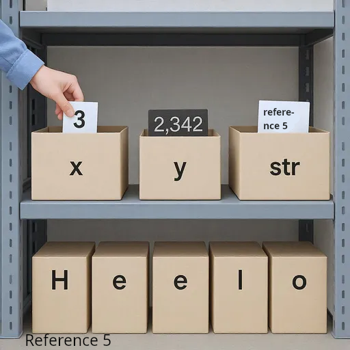
For example the command
x = 33stores the value 3 in the box tagged x.
Later, you may retrieve the value stored in the variable x, for example the command
x + 2528retrieves the value stored in x and adds 25 to it.
The assignment operator = is also used to assign the value (content) of one variable to another variable, or assign the result of a computation to a variable,
y=x
z=y+5
println("Now x = ", x, ", y = ", y, " and z = ",z, ".")
Now x = 3, y = 3 and z = 8.Algebraic operations on numbers
x = 3.0
y = 4.2
x*y, x+y, x-y, x/y, x^y
(12.600000000000001, 7.2, -1.2000000000000002, 0.7142857142857143, 100.90420610885693)u = 33
v =53.234
@show(u % 4) #u modulo 3
@show (u ÷ 7) #integer division without rest
@show (rem(u,7)) #this returns the rest after division
@show(v % 7)u % 4 = 1
u ÷ 7 = 4
rem(u, 7) = 5
v % 7 = 4.2340000000000024.234000000000002Mathematical functions
x = 2
√x #\sqrt + [TAB]1.4142135623730951sqrt(x)1.4142135623730951y = -x-2sqrt(y)DomainError with -2.0: sqrt was called with a negative real argument but will only return a complex result if called with a complex argument. Try sqrt(Complex(x)). Stacktrace: [1] throw_complex_domainerror(f::Symbol, x::Float64) @ Base.Math ./math.jl:33 [2] sqrt @ ./math.jl:627 [inlined] [3] sqrt(x::Int64) @ Base.Math ./math.jl:1546 [4] top-level scope @ ~/github/ProgrammingCourse-with-Julia-SimulationAnalysisAndLearningSystems/quarto/lecture-unit-1.qmd:211
z = sqrt(y + 0im)0.0 + 1.4142135623730951imLet’s see some mathematical in-built functions:
exp(1)2.718281828459045ℯ #\euler + [TAB],ℯ = 2.7182818284590...π #\pi + [TAB]π = 3.1415926535897...log(ℯ^2), log2(2^5), log10(10^3), sin(3π), cos(0.1), tan(π/3)(2.0, 5.0, 3.0, 3.6739403974420594e-16, 0.9950041652780258, 1.7320508075688767)abs(-3.5), abs(3.5), abs(3 + 4im)(3.5, 3.5, 5.0)factorial(4)24In Julia, there is special notation (“syntactic sugar”) for swapping values
If you do it in that naive way, then the following will happen.
%%{init: { 'flowchart': { 'scale': 0.7 } } }%%
flowchart LR
    x1([x]) -->  |step 1| y1([y])
    y1([y]) -->  |step 2| x1([x])
x = 20
y = 5

#swapping x and y:  attempt 1
x = y
y = x

@show x; #This is the @show macro
@show y;
x = 5
y = 5So the value in x is overwritten and lost as soon as it is overwritten by the value in y.
This can be fixed by storing the value in x temporarily in another variable.
%%{init: { 'flowchart': { 'scale': 0.7 } } }%%
flowchart LR
    x2([x]) -->  |step 1| temp([temp])
    y2([y]) -->  |step 2| x2([x])
    temp([temp]) --> |step 3| y2([y])
x = 20
y = 5

#swapping x and y:  attempt 2
temp = x
x = y
y = temp

@show x;
@show y;
x = 5
y = 20To simplify the notation for this, in Julia we can do it without using the variable temp:
x = 20
y = 5

x, y = y, x #Julia specific solution

@show x;
@show y;
x = 5
y = 20%%{init: { 'flowchart': { 'scale': 0.7 } } }%%
flowchart LR
x3([x,y]) --> |step 1| y3([y,x])
Variables have a type - think of it as the size and shape of the box. The command
typeof(x)Int64gives the type of the variable x (an integer value of size 8 bytes). The size can be obtained using the function sizeof, e.g.
sizeof(x)8The type Int64 is the standard type for integers. Particular integer numbers are written without .:
typeof(32)Int64Another big class of numeric variables are floating-point numbers. Specific floating-point numbers are written with a ., e.g.
y=34.23
typeof(y), sizeof(y)
(Float64, 8)defines a Floating point number of size 8 bytes = 64 bits. Floating point numbers are also the result when we divide integer numbers, e.g.
r=3/4
println(r)
typeof(r)0.75Float64and the result of many functions which typically return floating point numbers such as
result=cos(2)
result, typeof(result)
(-0.4161468365471424, Float64)Variables can not only contain numbers, but pretty much every type of data, for example letters and text. The data type of single letters is called Char, which is short for character. The values of type Char are written with simple ', for example
c = 'a'
typeof(c)Chary = 'η' # \eta + [TAB]
typeof(y), sizeof(y)(Char, 4)On the other hand, the data type for text is called String ("a string of characters!"). Keep in mind that double " are used to write Strings.
str = "Hello"
typeof(str)StringThe length of the string (number of characters) can be obtained from the built-in function length:
length(str)5But you can’t do absolute value of a string:
abs("3.5")MethodError: no method matching abs(::String) The function `abs` exists, but no method is defined for this combination of argument types. Closest candidates are: abs(::Bool) @ Base bool.jl:155 abs(::Pkg.Resolve.VersionWeight) @ Pkg ~/.julia/juliaup/julia-1.12.6+0.x64.linux.gnu/share/julia/stdlib/v1.12/Pkg/src/Resolve/versionweights.jl:32 abs(::Missing) @ Base missing.jl:101 ... Stacktrace: [1] top-level scope @ ~/github/ProgrammingCourse-with-Julia-SimulationAnalysisAndLearningSystems/quarto/lecture-unit-1.qmd:380
And for strings even some algebraic operations are defined,
s1 = "hello " #notice the extra space
s2 = "world"
@show typeof(s1);
s1*s2 #In Python it would have been x+y for concatenation
typeof(s1) = String"hello world"Even the exponential operator is defined for strings:
s = "hello "
y = 5
x^y3125These are examples of operator (method) overloading in Julia: For different data types, different versions of a function/method/operator can be defined.
s^(y-1)*s[1:end-1]"hello hello hello hello hello"Since the operator ^ has precedence of *, this is the same as
(s^(y-1))*s[1:end-1]"hello hello hello hello hello"What if we did the brackets the other way?
s^((y-1)*s[1:end-1])MethodError: no method matching *(::Int64, ::String) The function `*` exists, but no method is defined for this combination of argument types. Closest candidates are: *(::Any, ::Any, ::Any, ::Any...) @ Base operators.jl:642 *(::Missing, ::Union{AbstractChar, AbstractString}) @ Base missing.jl:174 *(::Real, ::Dates.Period) @ Dates ~/.julia/juliaup/julia-1.12.6+0.x64.linux.gnu/share/julia/stdlib/v1.12/Dates/src/periods.jl:91 ... Stacktrace: [1] top-level scope @ ~/github/ProgrammingCourse-with-Julia-SimulationAnalysisAndLearningSystems/quarto/lecture-unit-1.qmd:412
Here, Julia tries to identify an instance of the method “*(.,.)” which takes an Integer and a String as arguments (this is Julia’s “multiple dispatch” paradigm), but doesn’t succeed. The closest candidates are listed in the error message, but none of them fits (e.g., any argument of type Int64 can be converted into types Real, Number, Any, etc).
For type conversions, in particular between integers and floating point numbers, use Float64 and Int as though they were functions:
a=4;
x=Float64(a);
@show typeof(a) a;
@show typeof(x) x;
typeof(a) = Int64
a = 4
typeof(x) = Float64
x = 4.0y=sqrt(5);
b=round(y);
@show typeof(y) y;
@show typeof(b) b;typeof(y) = Float64
y = 2.23606797749979
typeof(b) = Float64
b = 2.0Here, b is still of type Float64. Only after applying Int it becomes an integer
basInt=Int(b)
@show basInt;
@show typeof(basInt);
basInt = 2
typeof(basInt) = Int64The standard method to convert numbers into Strings uses the function string (lowercase!). E.g.
a=3
f=3.333
str="A string which includes a="*string(a)*" and f="*string(f)
"A string which includes a=3 and f=3.333"As special type of type conversion is String interpolation using the symbol $ which automatically converts a variable (and even an entire expression) into a String and inserts it into an existing string, e.g.:
i = 234
f = pi/2
println("An example of an integer is i=$i and an example for a floating-point number is f=$f.")
An example of an integer is i=234 and an example for a floating-point number is f=1.5707963267948966.Particular characters in a String can be retrieved using indexing. Julia indexing is 1-based, i.e. index 1 refers to the first letter, etc., whereas in other programming languages the first entry has index 0 be default.
str2 = "This is an example string!""This is an example string!"The following diagram illustrates how to retrieve characters from a string by index:
String: "This is an example string!"

Index position (1-based):
   1  2  3  4  5  6  7  8  9 10 11 12 13 14 15 16 17 18 19 20 21 22 23 24 25 26
   T  h  i  s     i  s     a  n     e  x  a  m  p  l  e     s  t  r  i  n  g  !

Examples:
  str2[1]      →  'T'    (first character)
  str2[7]      →  's'    (character at index 7)
  str2[end]    →  '!'    (last character)
  str2[end-5:end]  →  "tring!"  (substring from index 20 to 25)
str2[10:15] → "nample" (substring from index 10 to 15)c1=str2[1]
println("The first letter in the string is: ", c1)
typeof(c1)The first letter in the string is: TCharc7=str2[7]
println("and the 7th letter in the string is: ", c7)and the 7th letter in the string is: sThe special index end can be used to the last character of the string
clast=str2[end]
println("and the final letter in the string is: ", clast)
and the final letter in the string is: !Once can even retrieve sub-sections of a string, which gives another string, e.g.
string_end=str2[end-5:end]
println("and the final section of length 6 is: ", string_end)
and the final section of length 6 is: tring!or
middle=str2[10:15]
println("and a middle section of length 6 is: ", middle)
and a middle section of length 6 is: n examAnother example of types of variables that admit indexing are vectors
u=[1,2,3]
u[2]=5
v=u
3-element Vector{Int64}:
1
5
3and matrices
M=[1 2 3; 4 5 6; 7 8 9]
M*v
3-element Vector{Int64}:
20
47
74M[1,1]=0
M*v3-element Vector{Int64}:
19
47
74Note that dealing with such higher-dimensional objects is one of the big strengths of Julia and will be discussed in the coming units. For now, vectors (and matrices) only serve as examples of composite variables.
A big difference between Strings on the one hand and collections such as Vectors as well as Matrices on the other hand is that Strings in Julia are immutable whereas Vectors and Matrices are mutable. This means that Strings can not be modified in hindsight, whereas Vectors (and Matrices) can be modified after creation.
str="Here, I am creating a string variable"
str[5]='c'
MethodError: no method matching setindex!(::String, ::Char, ::Int64) The function `setindex!` exists, but no method is defined for this combination of argument types. Stacktrace: [1] top-level scope @ ~/github/ProgrammingCourse-with-Julia-SimulationAnalysisAndLearningSystems/quarto/lecture-unit-1.qmd:540
This creates an error whereas for a Matrix
v=[1,2,3]
v[1]=10
@show(v)
M=[1.0 2.0 3; 4 5 6; 7 8 9]
M[1, 2]=200.0
@show(M)
v = [10, 2, 3]
M = [1.0 200.0 3.0; 4.0 5.0 6.0; 7.0 8.0 9.0]3×3 Matrix{Float64}:
1.0 200.0 3.0
4.0 5.0 6.0
7.0 8.0 9.0Variables of type String are more complex than those for simple numbers. They are composed of a sequence of simpler components of type Char. In particular, the length of a String can vary, and therefore also the amount of memory it occupies.
For these reasons, Strings are examples of composite types, while the simple datatypes such as those for basic integers and floating point numbers, and the one of characters are called primitive types. This can be verified using the built-in function isbits which returns true (a logical constant - see below) for primitive types, and false for composite types.
isbits(x), isbits(c), isbits(str)(true, true, false)This has important consequences for how variables are stored in memory. Variables of primitive types, i.e. for which the variable directly refers to the value of the variable, are stored IN the variable - “in the box” denoted by the name of the variable (see figure above).
Variables of composite types, on the other hand, such as Strings do not refer directly to their content, but to the address (reference, pointer) in memory where the content is stored. Think of the reference as the shelf number in the computer memory which plays the role of a storage facility. For example in the figure above, the String variable str contains the reference (address) 5 which is the position in memory where the actual string containing “Heelo” is stored
This has striking consequences. For example, when assigning the content of one primitive variable to another variable, only the content is copied
x=10
y=x
@show(y)
y = 1010so we can change the content of one variable without modifying the content of the other one.
x=100
println(y)10On the other hand, for a composite type such as vectors and matrices,
u=[1,2,3]
v=u
3-element Vector{Int64}:
1
2
3This defines a vector of length 3 and copies the reference to this vector from u into v.
When we modify the content of u using indexing, we also modify the content of v:
u[1]=10
@show(v)
v = [10, 2, 3]3-element Vector{Int64}:
10
2
3graph TD
subgraph vars ["Variable Names (Stack)"]
U["u"]
V["v"]
end
subgraph mem ["Memory (Heap)"]
VEC["[1, 2, 3]"]
end
U -->|reference| VEC
V -->|reference| VEC
style U fill:#667eea,stroke:#333,stroke-width:2px,color:#fff
style V fill:#667eea,stroke:#333,stroke-width:2px,color:#fff
style VEC fill:#FF6B6B,stroke:#333,stroke-width:2px,color:#fff
style vars fill:#f0f0f0,stroke:#999
style mem fill:#fff9e6,stroke:#999
The reason is that using indexing, we directly modify the section in memory, to which both references in u and in v are pointing.
The data type Bool has only two possible values,
true, false #In Python it is True and False (caps first letter)(true, false)typeof(true)BoolInternally, those two values are represented like the integer values 0 and 1 (actually in programming languages which are closer to the hardware representation of the program, this is exactly how logical values are treated).
@show Int(true);
@show Int(false);
Int(true) = 1
Int(false) = 05 == 2 + 3 # check for equalitytrue5 != 2 + 3 # check for not being equal (!=)falsefalse && false, false && true, true && false, true && true #logical AND(false, false, false, true)false || false, false || true, true || false, true || true #logical OR(false, true, true, true)(2 != 3) || (2 == 3)true!(2 == 3) # ! (not)trueLogical AND (&&) has precedence of logical OR (||) as can be seen in
true || false && falsetrueFor the next block, you need to have the package Random installed: To install it, change to package mode using ], and use add Random.
The REPL modes are
; to access the shell/terminal temporarily,? for help mode,] for package mode,using Random
x = rand(1:100) #random number within 1, 2, ..., 100
y = rand(1:100) #random number within 1, 2, ..., 100
@show x, y;
(x == y) || (x != y)(x, y) = (72, 95)truex < y, x<=y, x ≤ y, x > y, x ≥ y # \le or \ge + [TAB](true, true, true, false, false)(x == y) && (x != y)falsex=[1,2,3]
y=[1,2,3]
x==ytruecompares the content of x to the content of y. To check whether x and y are physically identical (same reference) use
@show x===y;
z=y
@show z===y;
x === y = false
z === y = true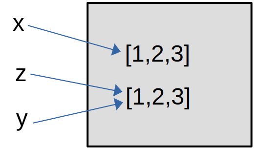
This is again a consequence of storage-by=reference. Initially the vector [1,2,3] is physically saved in memory twice. The reference to the first one is stored in the variable x, the reference to the second one is stored in y. For that reason the comparison x==y evaluates to true, this is because the content of the two vectors is equal. But when comparing the two variables using the comparison operator ===, the result is false, because physically the two variables “point to” two different positions in memory.
Note that for Strings the result is different,
s1="some text"
s2="some text"
@show(s1==s2)
@show(s1===s2)
s1 == s2 = true
s1 === s2 = truetruebecause Strings are immutable. This enables the compiler to optimise memory usage by storing the String constant "some text" only once in memory!
if-elseif-else)%%{init: { 'flowchart': { 'scale': 0.7 } } }%%
flowchart TD
Start([Start]) --> Cond1{if condition}
Cond1 -->|true| IfBlock["Execute if block"]
Cond1 -->|false| Cond2{elseif condition}
Cond2 -->|true| ElseIfBlock["Execute elseif block"]
Cond2 -->|false| ElseBlock["Execute else block"]
IfBlock --> End([End])
ElseIfBlock --> End
ElseBlock --> End
if 2 < 3 && 2 > 3
   println("The world has gone crazy")
end
if 2 < 3 || 2 > 3
println("The world makes sense")
endThe world makes sensex = 25.3
if x < 30
println("It is less than 30")
else
println("It is greater or equal to 30")
endIt is less than 30x = 25.3
if x < 20
println("It is less than 20")
elseif x < 30
println("It is less than 30 but not less than 20")
else
println("It is greater or equal to 30")
endIt is less than 30 but not less than 20Let’s use it to compute an absolute value.
x = -3 # some input
if x < 0
   println(-x)
else
   println(x)
end3Use either the ternary operator condition ? dothisiftrue : dothisiffalse
x = -3 # some input
absx = x < 0 ? -x : x3is the equivalten to
x = -3 # some input
if x<0
   absx=-x
else
   absx=x
end3or using logical AND (&&), making use of Julia’s lazy evalution of logical operators,
x = -3 # some input
x < 0 && println("This is a negative number!")
This is a negative number!Here, the second condition for the AND clause && is only evaluated if the first condition evaluates to true. Effectively this behaves like a single-line if statement.
You might want to execute a specific section of your code more than once, for example for a certain number of times, or until a condition is reached. The section of a program which is structured in this way is called a loop.
In principle, a loop can be implemented by combining an
%%{init: { 'flowchart': { 'scale': 0.7 } } }%%
flowchart TD
    Start([Start]) --> Label["<b>loop:</b>"]
    Label --> Check{<b>IF condition<br/>true?</b>}
    Check -->|Yes| End["<b>goto end</b>"]
    Check -->|No| Execute["Continue code execution<br>(loop body)"]
    Execute --> Goto["<b>goto loop</b>"]
    Goto --> Label
    End --> Label2["<b>end:</b>"]
    style Label fill:#e1f5ff
In many programming languages, particularly older ones, such goto statements exist, but they make code error-prone as well as hard to read and to maintain. For that reason more modern programming languages either don’t include any type of goto command, or just in the form of macros which is the case for Julia.
It is pretty much always better to implement loops through dedicated control structures, namely for loops and while loops.
%%{init: { 'flowchart': { 'scale': 0.7 } } }%%
flowchart LR
    Start([Start]) -->  Check{While condition<br/>true?}
    Check -->|Yes| Execute["Execute loop body"]
    Execute --> Check
    Check -->|No| End([End])
In while loops, the loop section is written as a while block with the termination condition (actually it should be rather called continuation condition) at the BEGINNING of the loop section. Any initialisation has to happen before the while loop.
i = 1
while i ≤ 3   # do the following as long as i is smaller or equal than 3
   global i
   println(i)
   i = i + 1
end
1
2
3In particular, if the continuation condition is never satisfied, the loop will not be executed, not even once.
i = 5
while i ≤ 3 # do the following as long as i is smaller or equal than 3
global i
println(i)
i = i + 1
endOn the other hand, once can also write infinite loops which by themself won’t terminante, unless the user presses Ctrl-C (or kills the program by some other method).
i=0
while true # do it forever!
global i
println(i)
i = i + 1
endAs an example, where we compute the beginning of the hailstone sequence: If a number is even, half it, if it is odd, multiply by 3 and add 1. Stop when you reach 1.
n = 7
while n != 1
#global n
print(n, ", ")
if n % 2 == 0 # modulo 2...testing of n is even
n = n ÷ 2 # \div + [TAB] Integer division
else
n = 3n + 1
end
end
println(n)7, 22, 11, 34, 17, 52, 26, 13, 40, 20, 10, 5, 16, 8, 4, 2, 1%%{init: { 'flowchart': { 'scale': 0.7 } } }%%
flowchart TD
Start([Start]) --> Init["Initialize loop iterator<br/>for i in collection"]
Init --> Check{More items<br/>in collection?}
Check -->|No| End([End])
Check -->|Yes| Assign["Assign current item to i"]
Assign --> Execute["Execute loop body"]
Execute --> Next["Move to next item"]
Next --> Check
In for loops, the loop section is written as a for...end block with a counter and an ordered index set in the for line at the beginning of the block.
The for line serves three functions:
for i in 2:5
println("hello nr ", i)
endhello nr 2
hello nr 3
hello nr 4
hello nr 5for i ∈ 1:3 # \in + [TAB]
println("hello nr ", i)
endhello nr 1
hello nr 2
hello nr 3If the counter is not used in the loop, then _ can be used as place holder:
for _ ∈ 1:3 # \in + [TAB]
println("hello")
endhello
hello
helloA more general way of writing thisis
for i in eachindex(1:3)
println("hello nr ", i)
endhello nr 1
hello nr 2
hello nr 3For example, summation of all elements in a finite sequence:
total = 0
max_val = 10
for i in 1:max_val
global total # This line can be ignored by now
total = total + i
end
println("The total is: $total")
println("And using a formula: ", max_val*(max_val+1)/2)The total is: 55
And using a formula: 55.0Notice the above 55 vs. 55.0. This is because of division which converts an integer to a float.
break and continue%%{init: { 'flowchart': { 'scale': 0.4 } } }%%
flowchart TD
LoopStart --> Check{Loop condition<br/>true?}
Check -->|No| LoopEnd["Loop ends"]
Check -->|Yes| Statement1["Execute first<br>statements in the loop"]
Statement1 --> Decision{Check condition<br/>for break/continue?}
Decision -->|break| LoopEnd
Decision -->|continue| Check
Decision -->|neither| Statement2["Execute remaining<br/>statements in loop"]
Statement2 --> Check
style LoopEnd fill:#ffcdd2
style Decision fill:#fff9c4
The archaic form or writing loops using if and some sort of goto command is arguably more flexible, and sometimes this type of flexibility is very helpful. For that reason, many programming languages such as Julia implement the commands continue and break by which the loop execution can be controlled from whithin the loop.
Using the command continue within a loop, code executation continues at the start of the loop.
for i in 1:13
if i<10
continue
else
println("hello ", i)
end
endhello 10
hello 11
hello 12
hello 13Using the command break within a loop, loops can be left at any time.
for i ∈ 1:13 # \in + [TAB]
if i<5
println("hello $i")
else
break
end
endhello 1
hello 2
hello 3
hello 4for i ∈ 1:13 # \in + [TAB]
if i>10
break
else
println("hello $i")
end
endhello 1
hello 2
hello 3
hello 4
hello 5
hello 6
hello 7
hello 8
hello 9
hello 10%%{init: { 'flowchart': { 'scale': 0.5 } } }%%
flowchart LR
Start([Start]) --> DoStuff["execute loop"]
DoStuff --> IfCond{"if condition"}
IfCond -->|true| Break["break"]
IfCond -->|false| DoStuff
Break --> End([End])
In do-while loops, the continuation condition is at the end of the loop. Therefore, the loop is executed at least once before the continuation condition is evaluated! No explicit syntax for do-while loops exists in Julia, since this particular behavior can be reproduced by combining an infinite while loop with if and break commands:
i=0
while true
# do stuff
println(i)
i = i + 1
if i>5
break
end
# shorter: i>5 || break
end0
1
2
3
4
5This is to demonstrate that with a do-while loop, the loop section is always executed at least once, even if the termination condition is true from the start:
i=10
while true
    # do stuff
    println(i)
    i = i + 1
    if i>5
      break
    end
    # shorter:  i>5 || break
end10%%{init: { 'flowchart': { 'scale': 0.5 } } }%%
flowchart TD
Start(["Call function"]) --> |arg1, arg2, arg3, ...|FuncStart["Function start"]
FuncStart --> Process["Do something with<br/>arguments"]
Process --> Check{Compute explicit<br> return-value?}
Check --> |Yes| Return("compute myreturnvalue")
Check --> |No| Default("take return-value of<br/>last executed statement")
Return --> |return myreturnvalue| End([Receive return-value])
Default --> |return it implicitly| End([Receive return-value])
We already had logic for an absolute value function (of real values). Now let’s make a callable function out of it:
function my_abs(x)
   if x < 0
      return -x
   else
      return x
   end
end
my_abs (generic function with 1 method)Note that using the command return the function terminates and the argument of the return command becomes the return value of the function. We can also implement this as,
function my_abs(x)
   if x < 0
      return -x
   end
   return x
end
my_abs (generic function with 1 method)Or even,
function my_abs(x)
   if x < 0
      return -x
   end
   x
end
my_abs (generic function with 1 method)which uses that functions by default return the output of the last command.
@show my_abs(-3.5);
@show my_abs(2.3);
@show my_abs(0);
my_abs(-3.5) = 3.5
my_abs(2.3) = 2.3
my_abs(0) = 0Functions don’t have to have an argument or a return value:
function print_my_details()
   println("Name: Jacob")
   println("Occupation: diesel mechanic")
   return nothing
end

print_my_details()
Name: Jacob
Occupation: diesel mechanicWhen you can implement a function in one line, you can avoid using the function keyword and instead use mathematical notation for defining functions:
Instead of
function times_1(x)
   return 2x
end
times_1(343)686you could also just define a function as follows:
times_2(x) = 2xtimes_2 (generic function with 1 method)These two function definitions are actually perfectly equivalent. Once functions are defined, you can for example compose them as follows:
@show times_2(times_2(10)) #this uses the function twice.
@show (times_2 ∘ times_2)(10) # \circ...alternative way of writing function composition
times_2(times_2(10)) = 40
(times_2 ∘ times_2)(10) = 4040Note that on many occasion when there is no ambiguity, Julia permits omitting the multiplication symbol * in order to mimic mathematical notation even more closely.
Let’s formulate the computation of the first 10 elements of the hailstone sequence as a function:
#here, we "wrap" the code we had before in a function
function hailstone(n_start)
   n = n_start
   while n != 1
      print(n, ", ")
      if n % 2 == 0 #is n even?
         n = n ÷ 2
      else
         n = 3n + 1
      end
   end
   println(n)
   return nothing
end

hailstone(7)
7, 22, 11, 34, 17, 52, 26, 13, 40, 20, 10, 5, 16, 8, 4, 2, 1Note that the function actually only outputs the elements of the hailstone sequence, but it doesn’t return them.
println("Hailstone sequences: ")
for n in 1:10
   hailstone(n)
end
Hailstone sequences:
1
2, 1
3, 10, 5, 16, 8, 4, 2, 1
4, 2, 1
5, 16, 8, 4, 2, 1
6, 3, 10, 5, 16, 8, 4, 2, 1
7, 22, 11, 34, 17, 52, 26, 13, 40, 20, 10, 5, 16, 8, 4, 2, 1
8, 4, 2, 1
9, 28, 14, 7, 22, 11, 34, 17, 52, 26, 13, 40, 20, 10, 5, 16, 8, 4, 2, 1
10, 5, 16, 8, 4, 2, 1The Collatz Conjecture says that for every starting value the sequence eventually hits 1. Let’s try to disprove it by seeing if this program gets stuck.
First I extend the definition of the function hailstone above, so it returns the length of the hailstone sequence rather than printing it.
function hailstone_length(n_start)
   n = n_start
   len = 1
   while n != 1
      len += 1 # short notation for n = n + 1
      # print(n, ", ")
      if n % 2 == 0
         n = n ÷ 2
      else
         n = 3n + 1
      end
   end
   #println(n)
   #println()
   return len
end

hailstone_length(7)17for n in 1:10^3
if n>1
print(", ")
end
print(hailstone_length(n))
end
println()1, 2, 8, 3, 6, 9, 17, 4, 20, 7, 15, 10, 10, 18, 18, 5, 13, 21, 21, 8, 8, 16, 16, 11, 24, 11, 112, 19, 19, 19, 107, 6, 27, 14, 14, 22, 22, 22, 35, 9, 110, 9, 30, 17, 17, 17, 105, 12, 25, 25, 25, 12, 12, 113, 113, 20, 33, 20, 33, 20, 20, 108, 108, 7, 28, 28, 28, 15, 15, 15, 103, 23, 116, 23, 15, 23, 23, 36, 36, 10, 23, 111, 111, 10, 10, 31, 31, 18, 31, 18, 93, 18, 18, 106, 106, 13, 119, 26, 26, 26, 26, 26, 88, 13, 39, 13, 101, 114, 114, 114, 70, 21, 13, 34, 34, 21, 21, 34, 34, 21, 96, 21, 47, 109, 109, 109, 47, 8, 122, 29, 29, 29, 29, 29, 42, 16, 91, 16, 42, 16, 16, 104, 104, 24, 117, 117, 117, 24, 24, 16, 16, 24, 37, 24, 86, 37, 37, 37, 55, 11, 99, 24, 24, 112, 112, 112, 68, 11, 50, 11, 125, 32, 32, 32, 81, 19, 32, 32, 32, 19, 19, 94, 94, 19, 45, 19, 45, 107, 107, 107, 45, 14, 120, 120, 120, 27, 27, 27, 120, 27, 19, 27, 40, 27, 27, 89, 89, 14, 40, 40, 40, 14, 14, 102, 102, 115, 27, 115, 53, 115, 115, 71, 71, 22, 53, 14, 14, 35, 35, 35, 128, 22, 84, 22, 128, 35, 35, 35, 53, 22, 22, 97, 97, 22, 22, 48, 48, 110, 48, 110, 66, 110, 110, 48, 48, 9, 123, 123, 123, 30, 30, 30, 79, 30, 123, 30, 22, 30, 30, 43, 43, 17, 30, 92, 92, 17, 17, 43, 43, 17, 43, 17, 61, 105, 105, 105, 43, 25, 30, 118, 118, 118, 118, 118, 56, 25, 74, 25, 118, 17, 17, 17, 43, 25, 38, 38, 38, 25, 25, 87, 87, 38, 131, 38, 38, 38, 38, 56, 56, 12, 25, 100, 100, 25, 25, 25, 144, 113, 51, 113, 25, 113, 113, 69, 69, 12, 113, 51, 51, 12, 12, 126, 126, 33, 126, 33, 126, 33, 33, 82, 82, 20, 126, 33, 33, 33, 33, 33, 51, 20, 46, 20, 46, 95, 95, 95, 46, 20, 20, 46, 46, 20, 20, 46, 46, 108, 64, 108, 59, 108, 108, 46, 46, 15, 33, 121, 121, 121, 121, 121, 121, 28, 59, 28, 77, 28, 28, 121, 121, 28, 20, 20, 20, 28, 28, 41, 41, 28, 41, 28, 134, 90, 90, 90, 134, 15, 134, 41, 41, 41, 41, 41, 33, 15, 59, 15, 54, 103, 103, 103, 41, 116, 28, 28, 28, 116, 116, 54, 54, 116, 28, 116, 54, 72, 72, 72, 98, 23, 116, 54, 54, 15, 15, 15, 41, 36, 129, 36, 129, 36, 36, 129, 129, 23, 36, 85, 85, 23, 23, 129, 129, 36, 36, 36, 28, 36, 36, 54, 54, 23, 49, 23, 23, 98, 98, 98, 142, 23, 49, 23, 142, 49, 49, 49, 98, 111, 23, 49, 49, 111, 111, 67, 67, 111, 62, 111, 36, 49, 49, 49, 62, 10, 36, 124, 124, 124, 124, 124, 62, 31, 124, 31, 124, 31, 31, 80, 80, 31, 31, 124, 124, 31, 31, 23, 23, 31, 23, 31, 49, 44, 44, 44, 137, 18, 44, 31, 31, 93, 93, 93, 44, 18, 137, 18, 31, 44, 44, 44, 88, 18, 44, 44, 44, 18, 18, 62, 62, 106, 57, 106, 31, 106, 106, 44, 44, 26, 31, 31, 31, 119, 119, 119, 31, 119, 57, 119, 119, 119, 119, 57, 57, 26, 75, 75, 75, 26, 26, 119, 119, 18, 57, 18, 70, 18, 18, 44, 44, 26, 132, 39, 39, 39, 39, 39, 70, 26, 132, 26, 132, 88, 88, 88, 132, 39, 26, 132, 132, 39, 39, 39, 39, 39, 31, 39, 31, 57, 57, 57, 132, 13, 52, 26, 26, 101, 101, 101, 39, 26, 145, 26, 101, 26, 26, 145, 145, 114, 52, 52, 52, 114, 114, 26, 26, 114, 52, 114, 145, 70, 70, 70, 96, 13, 65, 114, 114, 52, 52, 52, 65, 13, 65, 13, 39, 127, 127, 127, 39, 34, 127, 127, 127, 34, 34, 127, 127, 34, 127, 34, 65, 83, 83, 83, 171, 21, 34, 127, 127, 34, 34, 34, 65, 34, 26, 34, 26, 34, 34, 52, 52, 21, 47, 47, 47, 21, 21, 47, 47, 96, 34, 96, 140, 96, 96, 47, 47, 21, 140, 21, 21, 47, 47, 47, 96, 21, 91, 21, 47, 47, 47, 47, 140, 109, 21, 65, 65, 109, 109, 60, 60, 109, 34, 109, 153, 47, 47, 47, 60, 16, 34, 34, 34, 122, 122, 122, 153, 122, 34, 122, 60, 122, 122, 122, 122, 29, 122, 60, 60, 29, 29, 78, 78, 29, 78, 29, 104, 122, 122, 122, 73, 29, 60, 21, 21, 21, 21, 21, 73, 29, 47, 29, 135, 42, 42, 42, 135, 29, 42, 42, 42, 29, 29, 135, 135, 91, 135, 91, 42, 91, 91, 135, 135, 16, 29, 135, 135, 42, 42, 42, 86, 42, 42, 42, 42, 42, 42, 34, 34, 16, 60, 60, 60, 16, 16, 55, 55, 104, 29, 104, 148, 104, 104, 42, 42, 117, 148, 29, 29, 29, 29, 29, 179, 117, 148, 117, 29, 55, 55, 55, 148, 117, 117, 29, 29, 117, 117, 55, 55, 73, 148, 73, 47, 73, 73, 99, 99, 24, 68, 117, 117, 55, 55, 55, 117, 16, 68, 16, 55, 16, 16, 42, 42, 37, 130, 130, 130, 37, 37, 130, 130, 37, 130, 37, 68, 130, 130, 130, 117, 24, 130, 37, 37, 86, 86, 86, 130, 24, 174, 24, 86, 130, 130, 130, 37, 37, 37, 37, 37, 37, 37, 29, 29, 37, 29, 37, 29, 55, 55, 55, 130, 24, 50, 50, 50, 24, 24, 24, 143, 99, 50, 99, 37, 99, 99, 143, 143, 24, 99, 50, 50, 24, 24, 143, 143, 50, 24, 50, 37, 50, 50, 99, 99, 112, 94, 24, 24, 50, 50, 50, 50, 112It didn’t get stuck (try even changing 10^3 to 10^6). If the loop would “get stuck”, it wouldn’t terminate unless we press Ctrl-C!
Now let’s see what was the longest sequence.
length_of_longest = 0
n_of_longest = 0
for n in 1:10^3
   global length_of_longest, n_of_longest
   seq_len = hailstone_length(n)
   if seq_len > length_of_longest
      length_of_longest = seq_len
      n_of_longest = n
   end
end

println("The longest hailstone sequence is of length $length_of_longest when you start at $n_of_longest.")
The longest hailstone sequence is of length 179 when you start at 871.Write a function called fizz_buzz that accepts a number and
Write a Julia function which returns the number of spaces in the String provided as argument to the function. Test the function using the argument “Julia uses the Multiple-Dispatch paradigm!”
Rewrite the following piece of code
cn=1
println(cn)
for i=1:5
   cn=sin(cn)
   println(cn)
end
using a
while loop andif clause to mimic a do-while-loop. Aim at avoiding redundant statements, yet, both versions of the script should generate the exactly same output as the code above.Write a short script which prints the first 30 elements of the recursion relation \(c_{n+1}=4 c_n - 3 c_{n-1}\) starting with \(c_1=0\) and \(c_2=1\). At the end the script should also print the sum \(c_1+c_2+...c_{30}\).
Sum of squares: Write a function called sum_of_squares that accepts the natural number \(n\) and returns the sum \(1^2 + 2^2 + \cdots + (n-1)^2 + n^2\).
What is the type of each of the following Julia expressions?
3
3.0
'3'
3>0
"3"
Fibonacci Sequence: Calculate the first element of the Fibonacci sequence \(a_0 = 1, a_1 = 1, a_{n+2} = a_{n+1} + a_n\) greater than \(1000\), and store it in a variable called an.
Consider the Julia code:
a = [1, 4, 9]
s = a[1]*a[2]*a[3]
What is the type and value of s?
You want to write a function my_minimum that gets a vector of numbers and returns the minimal value in the array. Do not use the minimum in-built function as part of your answer.
You want to write a Julia function is_sub_str which accepts two Strings str and substr, and returns true is substr is a sub-string of str (do not use any library functions, but only the tools developed in this Unit 1).
Which of the following correctly defines a Julia function that returns the square of its argument?
square(x) = x*xfunction square(x)
x*x
endC. Both A and B
D. Neither
Consider the Julia function, tamid_nahon which gets two boolean values as inputs, a, and b.
function tamid_nahon(a, b)
   return !(a && b) == !a || !b
end
For what combinations of a and b is the return value true? For what is it false?
Write a function round_to_nearest_int that takes a floating-point number and returns it as an integer type, rounded to the nearest integer. Test it with values like 3.7, -2.3, and 5.5.
Without running the code, predict the output of the following expression and explain why:
result = true || false && falseWhat is the value of result? Where could you add parenthesis to change the result?
Write a Julia expression which computes the exponential of pi/2 and stores the result in a variable named res. What is the type of this variable?
Which operator tests whether two values are numerically equal?
A. =
B. ==
C. :=
D. ===
Write a script which asks the user to input a loginname and then prints a statement like the following: “Your loginname includes xxx integer numbers between 0 and 9”.
Write a function substrings which takes the String str as argument and returns three substrings, one which starts like str, one which ends like str and one take from somewhere in the middle. The lengths of these substrings should be random every time the function is executed.
Write a function count_down that takes a positive integer n and prints all numbers from n down to 1, each on a separate line, using a while loop. After printing all numbers, it should print “Liftoff!”.
What is printed?
A = [1, 2, 3]
B = A
B[2] = 100

println(A)
Write a function print_odd_numbers that takes an integer n and prints all odd numbers from 1 to n (inclusive). Use a for loop and the continue statement to skip even numbers.
Consider the Julia function
function myfun2(a)
   i=10
   while i<115
      if i >= a
         break
      end
      println(i)
      i = i+1
   end
   return i
end
A. What is the output written by println when calling myfun2(10)?
B. What is the return value of myfun2(11)?
What is printed?
str1 = "hello"
str2 = str1
str1 = "world"
println(str2)
Would the behavior be different if we used vectors instead of strings?
Consider the following code:
vec1 = [1, 2, 3]
vec2 = vec1
vec3 = [1, 2, 3]
Which of the following comparisons will return true and which will return false? Explain why.
vec1 == vec2vec1 === vec2vec1 == vec3vec1 === vec3Rewrite the following if-else statement using the ternary operator:
if x >= 0
   result = sqrt(x)
else
   result = 0.0
end
Write two functions: double(x) that returns 2*x and add_five(x) that returns x + 5. Then use function composition to create a single expression that first doubles a number and then adds five to the result.
Given name = "Julia", which expression produces Hello Julia!?
A. "Hello name!"
B. "Hello $name!"
C. 'Hello $name!'
D. println(name)
Write a function digit_sum that takes a positive integer n and returns the sum of its digits. For example, digit_sum(123) should return 6 (because 1 + 2 + 3 = 6). Hint: Use the modulo operator % and integer division ÷.
Write a function check_brackets that takes a string containing a mathematical expression and checks whether opening and closing brackets are balanced (i.e. for every opening bracked there is a closing one).
What is printed?
x = 5
if x > 3
   println("A")
elseif x > 5
   println("B")
else
   println("C")
end
What is printed?
s = 0
for i in 1:4
   s += i
end
println(s)
Write a Julia function is_even(n) that returns true if n is even and false otherwise.